Vector Autoregression (VAR) – Comprehensive Guide with Examples in Python

Vector Autoregression (VAR) is a forecasting algorithm that can be used when two or more time series influence each other. That is, the relationship between the time series involved is bi-directional. In this post, we will see the concepts, intuition behind VAR models and see a comprehensive and correct method to train and forecast VAR models in python using statsmodels.

Vector Autoregression (VAR) – Comprehensive Guide with Examples in Python. Photo by Kyran Low.

Content

Introduction
Intuition behind VAR Model Formula
Building a VAR model in Python
Import the datasets
Visualize the Time Series
Testing Causation using Granger’s Causality Test
Cointegration Test
Split the Series into Training and Testing Data
Check for Stationarity and Make the Time Series Stationary
How to Select the Order (P) of VAR model
Train the VAR Model of Selected Order(p)
Check for Serial Correlation of Residuals (Errors) using Durbin Watson Statistic
How to Forecast VAR model using statsmodels
Train the VAR Model of Selected Order(p)
Invert the transformation to get the real forecast
Plot of Forecast vs Actuals
Evaluate the Forecasts
Conclusion

1. Introduction

First, what is Vector Autoregression (VAR) and when to use it?

Vector Autoregression (VAR) is a multivariate forecasting algorithm that is used when two or more time series influence each other.

That means, the basic requirements in order to use VAR are:

You need at least two time series (variables)
The time series should influence each other.

Alright. So why is it called ‘Autoregressive’?

It is considered as an Autoregressive model because, each variable (Time Series) is modeled as a function of the past values, that is the predictors are nothing but the lags (time delayed value) of the series.

Ok, so how is VAR different from other Autoregressive models like AR, ARMA or ARIMA?

The primary difference is those models are uni-directional, where, the predictors influence the Y and not vice-versa. Whereas, Vector Auto Regression (VAR) is bi-directional. That is, the variables influence each other.

We will go more in detail in the next section.

In this article you will gain a clear understanding of:

Intuition behind VAR Model formula
How to check the bi-directional relationship using Granger Causality
Procedure to building a VAR model in Python
How to determine the right order of VAR model
Interpreting the results of VAR model
How to generate forecasts to original scale of time series

2. Intuition behind VAR Model Formula

If you remember in Autoregression models, the time series is modeled as a linear combination of it’s own lags. That is, the past values of the series are used to forecast the current and future.

A typical AR(p) model equation looks something like this:

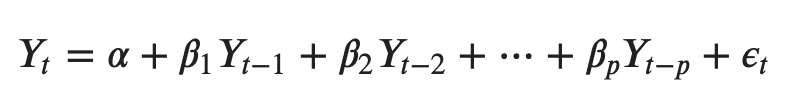
where α is the intercept, a constant and β1, β2 till βp are the coefficients of the lags of Y till order p.

Order ‘p’ means, up to p-lags of Y is used and they are the predictors in the equation. The ε_{t} is the error, which is considered as white noise.

Alright. So, how does a VAR model’s formula look like?

In the VAR model, each variable is modeled as a linear combination of past values of itself and the past values of other variables in the system. Since you have multiple time series that influence each other, it is modeled as a system of equations with one equation per variable (time series).

That is, if you have 5 time series that influence each other, we will have a system of 5 equations.

Well, how is the equation exactly framed?

Let’s suppose, you have two variables (Time series) Y1 and Y2, and you need to forecast the values of these variables at time (t).

To calculate Y1(t), VAR will use the past values of both Y1 as well as Y2. Likewise, to compute Y2(t), the past values of both Y1 and Y2 be used.

For example, the system of equations for a VAR(1) model with two time series (variables `Y1` and `Y2`) is as follows:

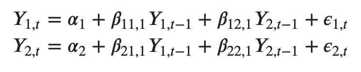
Where, Y{1,t-1} and Y{2,t-1} are the first lag of time series Y1 and Y2 respectively.

The above equation is referred to as a VAR(1) model, because, each equation is of order 1, that is, it contains up to one lag of each of the predictors (Y1 and Y2).

Since the Y terms in the equations are interrelated, the Y’s are considered as endogenous variables, rather than as exogenous predictors.

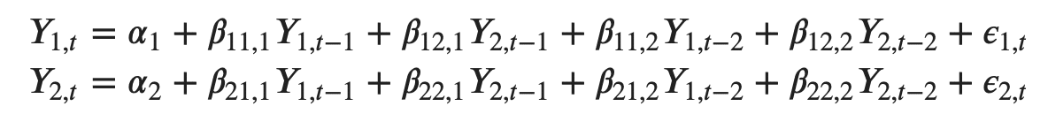
Likewise, the second order VAR(2) model for two variables would include up to two lags for each variable (Y1 and Y2).

Can you imagine what a second order VAR(2) model with three variables (Y1, Y2 and Y3) would look like?

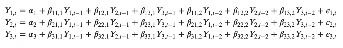
As you increase the number of time series (variables) in the model the system of equations become larger.

3. Building a VAR model in Python

The procedure to build a VAR model involves the following steps:

Analyze the time series characteristics
Test for causation amongst the time series
Test for stationarity
Transform the series to make it stationary, if needed
Find optimal order (p)
Prepare training and test datasets
Train the model
Roll back the transformations, if any.
Evaluate the model using test set
Forecast to future

import pandas as pd
import numpy as np
import matplotlib.pyplot as plt
%matplotlib inline

# Import Statsmodels
from statsmodels.tsa.api import VAR
from statsmodels.tsa.stattools import adfuller
from statsmodels.tools.eval_measures import rmse, aic

4. Import the datasets

For this article let’s use the time series used in Yash P Mehra’s 1994 article: “Wage Growth and the Inflation Process: An Empirical Approach”.

This dataset has the following 8 quarterly time series:

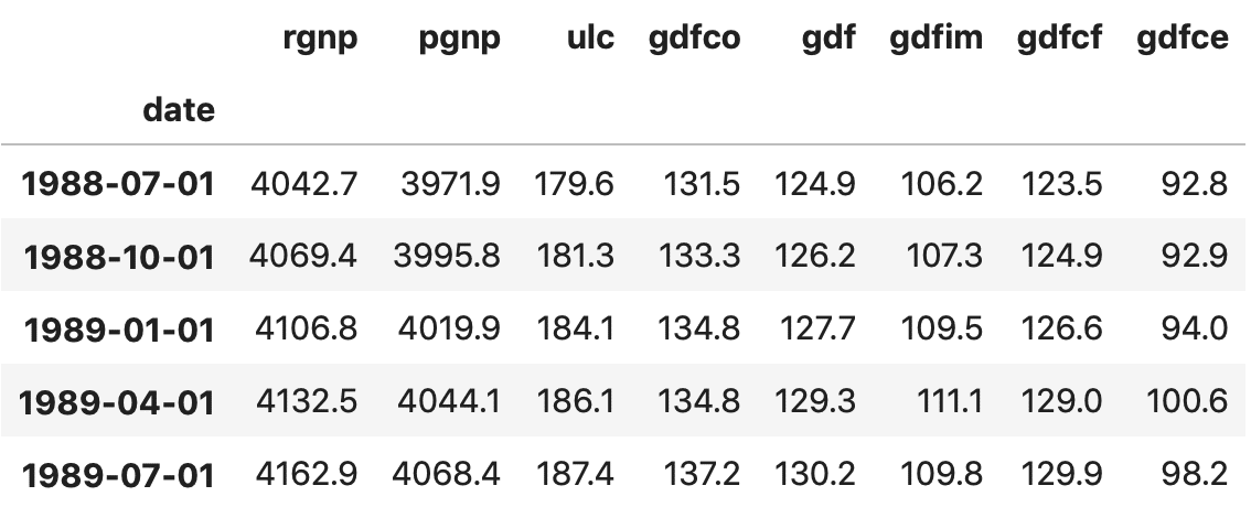
1. rgnp  : Real GNP.
2. pgnp  : Potential real GNP.
3. ulc   : Unit labor cost.
4. gdfco : Fixed weight deflator for personal consumption expenditure excluding food and energy.
5. gdf   : Fixed weight GNP deflator.
6. gdfim : Fixed weight import deflator.
7. gdfcf : Fixed weight deflator for food in personal consumption expenditure.
8. gdfce : Fixed weight deflator for energy in personal consumption expenditure.

Let’s import the data.

filepath = 'https://raw.githubusercontent.com/selva86/datasets/master/Raotbl6.csv'
df = pd.read_csv(filepath, parse_dates=['date'], index_col='date')
print(df.shape)  # (123, 8)
df.tail()

5. Visualize the Time Series

# Plot
fig, axes = plt.subplots(nrows=4, ncols=2, dpi=120, figsize=(10,6))
for i, ax in enumerate(axes.flatten()):
    data = df[df.columns[i]]
    ax.plot(data, color='red', linewidth=1)
    # Decorations
    ax.set_title(df.columns[i])
    ax.xaxis.set_ticks_position('none')
    ax.yaxis.set_ticks_position('none')
    ax.spines["top"].set_alpha(0)
    ax.tick_params(labelsize=6)

plt.tight_layout();

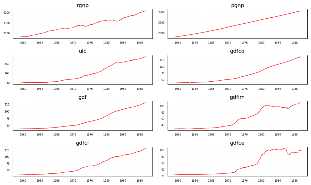
Actual Multi Dimensional Time Series for VAR model

Each of the series have a fairly similar trend patterns over the years except for gdfce and gdfim, where a different pattern is noticed starting in 1980.

Alright, next step in the analysis is to check for causality amongst these series. The Granger’s Causality test and the Cointegration test can help us with that.

6. Testing Causation using Granger’s Causality Test

The basis behind Vector AutoRegression is that each of the time series in the system influences each other. That is, you can predict the series with past values of itself along with other series in the system.

Using Granger’s Causality Test, it’s possible to test this relationship before even building the model.

So what does Granger’s Causality really test?

Granger’s causality tests the null hypothesis that the coefficients of past values in the regression equation is zero.

In simpler terms, the past values of time series (X) do not cause the other series (Y). So, if the p-value obtained from the test is lesser than the significance level of 0.05, then, you can safely reject the null hypothesis.

The below code implements the Granger’s Causality test for all possible combinations of the time series in a given dataframe and stores the p-values of each combination in the output matrix.

from statsmodels.tsa.stattools import grangercausalitytests
maxlag=12
test = 'ssr_chi2test'
def grangers_causation_matrix(data, variables, test='ssr_chi2test', verbose=False):    
    """Check Granger Causality of all possible combinations of the Time series.
    The rows are the response variable, columns are predictors. The values in the table 
    are the P-Values. P-Values lesser than the significance level (0.05), implies 
    the Null Hypothesis that the coefficients of the corresponding past values is 
    zero, that is, the X does not cause Y can be rejected.

    data      : pandas dataframe containing the time series variables
    variables : list containing names of the time series variables.
    """
    df = pd.DataFrame(np.zeros((len(variables), len(variables))), columns=variables, index=variables)
    for c in df.columns:
        for r in df.index:
            test_result = grangercausalitytests(data[[r, c]], maxlag=maxlag, verbose=False)
            p_values = [round(test_result[i+1][0][test][1],4) for i in range(maxlag)]
            if verbose: print(f'Y = {r}, X = {c}, P Values = {p_values}')
            min_p_value = np.min(p_values)
            df.loc[r, c] = min_p_value
    df.columns = [var + '_x' for var in variables]
    df.index = [var + '_y' for var in variables]
    return df

grangers_causation_matrix(df, variables = df.columns)

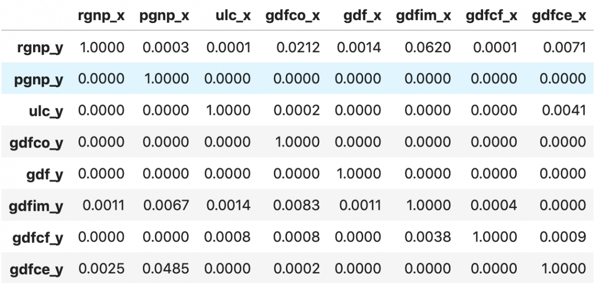
So how to read the above output?

The row are the Response (Y) and the columns are the predictor series (X).

For example, if you take the value 0.0003 in (row 1, column 2), it refers to the p-value of pgnp_x causing rgnp_y. Whereas, the 0.000 in (row 2, column 1) refers to the p-value of rgnp_y causing pgnp_x.

So, how to interpret the p-values?

If a given p-value is < significance level (0.05), then, the corresponding X series (column) causes the Y (row).

For example, P-Value of 0.0003 at (row 1, column 2) represents the p-value of the Grangers Causality test for pgnp_x causing rgnp_y, which is less that the significance level of 0.05.

So, you can reject the null hypothesis and conclude pgnp_x causes rgnp_y.

Looking at the P-Values in the above table, you can pretty much observe that all the variables (time series) in the system are interchangeably causing each other.

This makes this system of multi time series a good candidate for using VAR models to forecast.

Next, let’s do the Cointegration test.

7. Cointegration Test

Cointegration test helps to establish the presence of a statistically significant connection between two or more time series.

But, what does Cointegration mean?

To understand that, you first need to know what is ‘order of integration’ (d).

Order of integration(d) is nothing but the number of differencing required to make a non-stationary time series stationary.

Now, when you have two or more time series, and there exists a linear combination of them that has an order of integration (d) less than that of the individual series, then the collection of series is said to be cointegrated.

Ok?

When two or more time series are cointegrated, it means they have a long run, statistically significant relationship.

This is the basic premise on which Vector Autoregression(VAR) models is based on. So, it’s fairly common to implement the cointegration test before starting to build VAR models.

Alright, So how to do this test?

Soren Johanssen in his paper (1991) devised a procedure to implement the cointegration test.

It is fairly straightforward to implement in python’s statsmodels, as you can see below.

from statsmodels.tsa.vector_ar.vecm import coint_johansen

def cointegration_test(df, alpha=0.05): 
    """Perform Johanson's Cointegration Test and Report Summary"""
    out = coint_johansen(df,-1,5)
    d = {'0.90':0, '0.95':1, '0.99':2}
    traces = out.lr1
    cvts = out.cvt[:, d[str(1-alpha)]]
    def adjust(val, length= 6): return str(val).ljust(length)

    # Summary
    print('Name   ::  Test Stat > C(95%)    =>   Signif  \n', '--'*20)
    for col, trace, cvt in zip(df.columns, traces, cvts):
        print(adjust(col), ':: ', adjust(round(trace,2), 9), ">", adjust(cvt, 8), ' =>  ' , trace > cvt)

cointegration_test(df)

Results:

Name   ::  Test Stat > C(95%)    =>   Signif  
 ----------------------------------------
rgnp   ::  248.0     > 143.6691  =>   True
pgnp   ::  183.12    > 111.7797  =>   True
ulc    ::  130.01    > 83.9383   =>   True
gdfco  ::  85.28     > 60.0627   =>   True
gdf    ::  55.05     > 40.1749   =>   True
gdfim  ::  31.59     > 24.2761   =>   True
gdfcf  ::  14.06     > 12.3212   =>   True
gdfce  ::  0.45      > 4.1296    =>   False

8. Split the Series into Training and Testing Data

Splitting the dataset into training and test data.

The VAR model will be fitted on df_train and then used to forecast the next 4 observations. These forecasts will be compared against the actuals present in test data.

To do the comparisons, we will use multiple forecast accuracy metrics, as seen later in this article.

nobs = 4
df_train, df_test = df[0:-nobs], df[-nobs:]

# Check size
print(df_train.shape)  # (119, 8)
print(df_test.shape)  # (4, 8)

9. Check for Stationarity and Make the Time Series Stationary

Since the VAR model requires the time series you want to forecast to be stationary, it is customary to check all the time series in the system for stationarity.

Just to refresh, a stationary time series is one whose characteristics like mean and variance does not change over time.

So, how to test for stationarity?

There is a suite of tests called unit-root tests. The popular ones are:

Let’s use the ADF test for our purpose.

By the way, if a series is found to be non-stationary, you make it stationary by differencing the series once and repeat the test again until it becomes stationary.

Since, differencing reduces the length of the series by 1 and since all the time series has to be of the same length, you need to difference all the series in the system if you choose to difference at all.

Got it?

Let’s implement the ADF Test.

First, we implement a nice function (adfuller_test()) that writes out the results of the ADF test for any given time series and implement this function on each series one-by-one.

def adfuller_test(series, signif=0.05, name='', verbose=False):
    """Perform ADFuller to test for Stationarity of given series and print report"""
    r = adfuller(series, autolag='AIC')
    output = {'test_statistic':round(r[0], 4), 'pvalue':round(r[1], 4), 'n_lags':round(r[2], 4), 'n_obs':r[3]}
    p_value = output['pvalue'] 
    def adjust(val, length= 6): return str(val).ljust(length)

    # Print Summary
    print(f'    Augmented Dickey-Fuller Test on "{name}"', "\n   ", '-'*47)
    print(f' Null Hypothesis: Data has unit root. Non-Stationary.')
    print(f' Significance Level    = {signif}')
    print(f' Test Statistic        = {output["test_statistic"]}')
    print(f' No. Lags Chosen       = {output["n_lags"]}')

    for key,val in r[4].items():
        print(f' Critical value {adjust(key)} = {round(val, 3)}')

    if p_value <= signif:
        print(f" => P-Value = {p_value}. Rejecting Null Hypothesis.")
        print(f" => Series is Stationary.")
    else:
        print(f" => P-Value = {p_value}. Weak evidence to reject the Null Hypothesis.")
        print(f" => Series is Non-Stationary.")

Call the adfuller_test() on each series.

# ADF Test on each column
for name, column in df_train.iteritems():
    adfuller_test(column, name=column.name)
    print('\n')

Results:

    Augmented Dickey-Fuller Test on "rgnp" 
    -----------------------------------------------
 Null Hypothesis: Data has unit root. Non-Stationary.
 Significance Level    = 0.05
 Test Statistic        = 0.5428
 No. Lags Chosen       = 2
 Critical value 1%     = -3.488
 Critical value 5%     = -2.887
 Critical value 10%    = -2.58
 => P-Value = 0.9861. Weak evidence to reject the Null Hypothesis.
 => Series is Non-Stationary.


    Augmented Dickey-Fuller Test on "pgnp" 
    -----------------------------------------------
 Null Hypothesis: Data has unit root. Non-Stationary.
 Significance Level    = 0.05
 Test Statistic        = 1.1556
 No. Lags Chosen       = 1
 Critical value 1%     = -3.488
 Critical value 5%     = -2.887
 Critical value 10%    = -2.58
 => P-Value = 0.9957. Weak evidence to reject the Null Hypothesis.
 => Series is Non-Stationary.


    Augmented Dickey-Fuller Test on "ulc" 
    -----------------------------------------------
 Null Hypothesis: Data has unit root. Non-Stationary.
 Significance Level    = 0.05
 Test Statistic        = 1.2474
 No. Lags Chosen       = 2
 Critical value 1%     = -3.488
 Critical value 5%     = -2.887
 Critical value 10%    = -2.58
 => P-Value = 0.9963. Weak evidence to reject the Null Hypothesis.
 => Series is Non-Stationary.


    Augmented Dickey-Fuller Test on "gdfco" 
    -----------------------------------------------
 Null Hypothesis: Data has unit root. Non-Stationary.
 Significance Level    = 0.05
 Test Statistic        = 1.1954
 No. Lags Chosen       = 3
 Critical value 1%     = -3.489
 Critical value 5%     = -2.887
 Critical value 10%    = -2.58
 => P-Value = 0.996. Weak evidence to reject the Null Hypothesis.
 => Series is Non-Stationary.


    Augmented Dickey-Fuller Test on "gdf" 
    -----------------------------------------------
 Null Hypothesis: Data has unit root. Non-Stationary.
 Significance Level    = 0.05
 Test Statistic        = 1.676
 No. Lags Chosen       = 7
 Critical value 1%     = -3.491
 Critical value 5%     = -2.888
 Critical value 10%    = -2.581
 => P-Value = 0.9981. Weak evidence to reject the Null Hypothesis.
 => Series is Non-Stationary.


    Augmented Dickey-Fuller Test on "gdfim" 
    -----------------------------------------------
 Null Hypothesis: Data has unit root. Non-Stationary.
 Significance Level    = 0.05
 Test Statistic        = -0.0799
 No. Lags Chosen       = 1
 Critical value 1%     = -3.488
 Critical value 5%     = -2.887
 Critical value 10%    = -2.58
 => P-Value = 0.9514. Weak evidence to reject the Null Hypothesis.
 => Series is Non-Stationary.


    Augmented Dickey-Fuller Test on "gdfcf" 
    -----------------------------------------------
 Null Hypothesis: Data has unit root. Non-Stationary.
 Significance Level    = 0.05
 Test Statistic        = 1.4395
 No. Lags Chosen       = 8
 Critical value 1%     = -3.491
 Critical value 5%     = -2.888
 Critical value 10%    = -2.581
 => P-Value = 0.9973. Weak evidence to reject the Null Hypothesis.
 => Series is Non-Stationary.


    Augmented Dickey-Fuller Test on "gdfce" 
    -----------------------------------------------
 Null Hypothesis: Data has unit root. Non-Stationary.
 Significance Level    = 0.05
 Test Statistic        = -0.3402
 No. Lags Chosen       = 8
 Critical value 1%     = -3.491
 Critical value 5%     = -2.888
 Critical value 10%    = -2.581
 => P-Value = 0.9196. Weak evidence to reject the Null Hypothesis.
 => Series is Non-Stationary.

The ADF test confirms none of the time series is stationary. Let’s difference all of them once and check again.

# 1st difference
df_differenced = df_train.diff().dropna()

Re-run ADF test on each differenced series.

# ADF Test on each column of 1st Differences Dataframe
for name, column in df_differenced.iteritems():
    adfuller_test(column, name=column.name)
    print('\n')

    Augmented Dickey-Fuller Test on "rgnp" 
    -----------------------------------------------
 Null Hypothesis: Data has unit root. Non-Stationary.
 Significance Level    = 0.05
 Test Statistic        = -5.3448
 No. Lags Chosen       = 1
 Critical value 1%     = -3.488
 Critical value 5%     = -2.887
 Critical value 10%    = -2.58
 => P-Value = 0.0. Rejecting Null Hypothesis.
 => Series is Stationary.


    Augmented Dickey-Fuller Test on "pgnp" 
    -----------------------------------------------
 Null Hypothesis: Data has unit root. Non-Stationary.
 Significance Level    = 0.05
 Test Statistic        = -1.8282
 No. Lags Chosen       = 0
 Critical value 1%     = -3.488
 Critical value 5%     = -2.887
 Critical value 10%    = -2.58
 => P-Value = 0.3666. Weak evidence to reject the Null Hypothesis.
 => Series is Non-Stationary.


    Augmented Dickey-Fuller Test on "ulc" 
    -----------------------------------------------
 Null Hypothesis: Data has unit root. Non-Stationary.
 Significance Level    = 0.05
 Test Statistic        = -3.4658
 No. Lags Chosen       = 1
 Critical value 1%     = -3.488
 Critical value 5%     = -2.887
 Critical value 10%    = -2.58
 => P-Value = 0.0089. Rejecting Null Hypothesis.
 => Series is Stationary.


    Augmented Dickey-Fuller Test on "gdfco" 
    -----------------------------------------------
 Null Hypothesis: Data has unit root. Non-Stationary.
 Significance Level    = 0.05
 Test Statistic        = -1.4385
 No. Lags Chosen       = 2
 Critical value 1%     = -3.489
 Critical value 5%     = -2.887
 Critical value 10%    = -2.58
 => P-Value = 0.5637. Weak evidence to reject the Null Hypothesis.
 => Series is Non-Stationary.


    Augmented Dickey-Fuller Test on "gdf" 
    -----------------------------------------------
 Null Hypothesis: Data has unit root. Non-Stationary.
 Significance Level    = 0.05
 Test Statistic        = -1.1289
 No. Lags Chosen       = 2
 Critical value 1%     = -3.489
 Critical value 5%     = -2.887
 Critical value 10%    = -2.58
 => P-Value = 0.7034. Weak evidence to reject the Null Hypothesis.
 => Series is Non-Stationary.


    Augmented Dickey-Fuller Test on "gdfim" 
    -----------------------------------------------
 Null Hypothesis: Data has unit root. Non-Stationary.
 Significance Level    = 0.05
 Test Statistic        = -4.1256
 No. Lags Chosen       = 0
 Critical value 1%     = -3.488
 Critical value 5%     = -2.887
 Critical value 10%    = -2.58
 => P-Value = 0.0009. Rejecting Null Hypothesis.
 => Series is Stationary.


    Augmented Dickey-Fuller Test on "gdfcf" 
    -----------------------------------------------
 Null Hypothesis: Data has unit root. Non-Stationary.
 Significance Level    = 0.05
 Test Statistic        = -2.0545
 No. Lags Chosen       = 7
 Critical value 1%     = -3.491
 Critical value 5%     = -2.888
 Critical value 10%    = -2.581
 => P-Value = 0.2632. Weak evidence to reject the Null Hypothesis.
 => Series is Non-Stationary.


    Augmented Dickey-Fuller Test on "gdfce" 
    -----------------------------------------------
 Null Hypothesis: Data has unit root. Non-Stationary.
 Significance Level    = 0.05
 Test Statistic        = -3.1543
 No. Lags Chosen       = 7
 Critical value 1%     = -3.491
 Critical value 5%     = -2.888
 Critical value 10%    = -2.581
 => P-Value = 0.0228. Rejecting Null Hypothesis.
 => Series is Stationary.

After the first difference, Real Wages (Manufacturing) is still not stationary. It’s critical value is between 5% and 10% significance level.

All of the series in the VAR model should have the same number of observations.

So, we are left with one of two choices.

That is, either proceed with 1st differenced series or difference all the series one more time.

# Second Differencing
df_differenced = df_differenced.diff().dropna()

Re-run ADF test again on each second differenced series.

# ADF Test on each column of 2nd Differences Dataframe
for name, column in df_differenced.iteritems():
    adfuller_test(column, name=column.name)
    print('\n')

Results:

    Augmented Dickey-Fuller Test on "rgnp" 
    -----------------------------------------------
 Null Hypothesis: Data has unit root. Non-Stationary.
 Significance Level    = 0.05
 Test Statistic        = -9.0123
 No. Lags Chosen       = 2
 Critical value 1%     = -3.489
 Critical value 5%     = -2.887
 Critical value 10%    = -2.58
 => P-Value = 0.0. Rejecting Null Hypothesis.
 => Series is Stationary.


    Augmented Dickey-Fuller Test on "pgnp" 
    -----------------------------------------------
 Null Hypothesis: Data has unit root. Non-Stationary.
 Significance Level    = 0.05
 Test Statistic        = -10.9813
 No. Lags Chosen       = 0
 Critical value 1%     = -3.488
 Critical value 5%     = -2.887
 Critical value 10%    = -2.58
 => P-Value = 0.0. Rejecting Null Hypothesis.
 => Series is Stationary.


    Augmented Dickey-Fuller Test on "ulc" 
    -----------------------------------------------
 Null Hypothesis: Data has unit root. Non-Stationary.
 Significance Level    = 0.05
 Test Statistic        = -8.769
 No. Lags Chosen       = 2
 Critical value 1%     = -3.489
 Critical value 5%     = -2.887
 Critical value 10%    = -2.58
 => P-Value = 0.0. Rejecting Null Hypothesis.
 => Series is Stationary.


    Augmented Dickey-Fuller Test on "gdfco" 
    -----------------------------------------------
 Null Hypothesis: Data has unit root. Non-Stationary.
 Significance Level    = 0.05
 Test Statistic        = -7.9102
 No. Lags Chosen       = 3
 Critical value 1%     = -3.49
 Critical value 5%     = -2.887
 Critical value 10%    = -2.581
 => P-Value = 0.0. Rejecting Null Hypothesis.
 => Series is Stationary.


    Augmented Dickey-Fuller Test on "gdf" 
    -----------------------------------------------
 Null Hypothesis: Data has unit root. Non-Stationary.
 Significance Level    = 0.05
 Test Statistic        = -10.0351
 No. Lags Chosen       = 1
 Critical value 1%     = -3.489
 Critical value 5%     = -2.887
 Critical value 10%    = -2.58
 => P-Value = 0.0. Rejecting Null Hypothesis.
 => Series is Stationary.


    Augmented Dickey-Fuller Test on "gdfim" 
    -----------------------------------------------
 Null Hypothesis: Data has unit root. Non-Stationary.
 Significance Level    = 0.05
 Test Statistic        = -9.4059
 No. Lags Chosen       = 1
 Critical value 1%     = -3.489
 Critical value 5%     = -2.887
 Critical value 10%    = -2.58
 => P-Value = 0.0. Rejecting Null Hypothesis.
 => Series is Stationary.


    Augmented Dickey-Fuller Test on "gdfcf" 
    -----------------------------------------------
 Null Hypothesis: Data has unit root. Non-Stationary.
 Significance Level    = 0.05
 Test Statistic        = -6.922
 No. Lags Chosen       = 5
 Critical value 1%     = -3.491
 Critical value 5%     = -2.888
 Critical value 10%    = -2.581
 => P-Value = 0.0. Rejecting Null Hypothesis.
 => Series is Stationary.


    Augmented Dickey-Fuller Test on "gdfce" 
    -----------------------------------------------
 Null Hypothesis: Data has unit root. Non-Stationary.
 Significance Level    = 0.05
 Test Statistic        = -5.1732
 No. Lags Chosen       = 8
 Critical value 1%     = -3.492
 Critical value 5%     = -2.889
 Critical value 10%    = -2.581
 => P-Value = 0.0. Rejecting Null Hypothesis.
 => Series is Stationary.

All the series are now stationary.

Let’s prepare the training and test datasets.

10. How to Select the Order (P) of VAR model

To select the right order of the VAR model, we iteratively fit increasing orders of VAR model and pick the order that gives a model with least AIC.

Though the usual practice is to look at the AIC, you can also check other best fit comparison estimates of BIC, FPE and HQIC.

model = VAR(df_differenced)
for i in [1,2,3,4,5,6,7,8,9]:
    result = model.fit(i)
    print('Lag Order =', i)
    print('AIC : ', result.aic)
    print('BIC : ', result.bic)
    print('FPE : ', result.fpe)
    print('HQIC: ', result.hqic, '\n')

Results:

Lag Order = 1
AIC :  -1.3679402315450664
BIC :  0.3411847146588838
FPE :  0.2552682517347198
HQIC:  -0.6741331335699554 

Lag Order = 2
AIC :  -1.621237394447824
BIC :  1.6249432095295848
FPE :  0.2011349437137139
HQIC:  -0.3036288826795923 

Lag Order = 3
AIC :  -1.7658008387012791
BIC :  3.0345473163767833
FPE :  0.18125103746164364
HQIC:  0.18239143783963296 

Lag Order = 4
AIC :  -2.000735164470318
BIC :  4.3712151376540875
FPE :  0.15556966521481097
HQIC:  0.5849359332771069 

Lag Order = 5
AIC :  -1.9619535608363954
BIC :  5.9993645622420955
FPE :  0.18692794389114886
HQIC:  1.268206331178333 

Lag Order = 6
AIC :  -2.3303386524829053
BIC :  7.2384526890885805
FPE :  0.16380374017443664
HQIC:  1.5514371669548073 

Lag Order = 7
AIC :  -2.592331352347129
BIC :  8.602387254937796
FPE :  0.1823868583715414
HQIC:  1.9483069621146551 

Lag Order = 8
AIC :  -3.317261976458205
BIC :  9.52219581032303
FPE :  0.15573163248209088
HQIC:  1.8896071386220985 

Lag Order = 9
AIC :  -4.804763125958631
BIC :  9.698613139231597
FPE :  0.08421466682671915
HQIC:  1.0758291640834052

In the above output, the AIC drops to lowest at lag 4, then increases at lag 5 and then continuously drops further.

Let’s go with the lag 4 model.

An alternate method to choose the order(p) of the VAR models is to use the model.select_order(maxlags) method.

The selected order(p) is the order that gives the lowest ‘AIC’, ‘BIC’, ‘FPE’ and ‘HQIC’ scores.

x = model.select_order(maxlags=12)
x.summary()

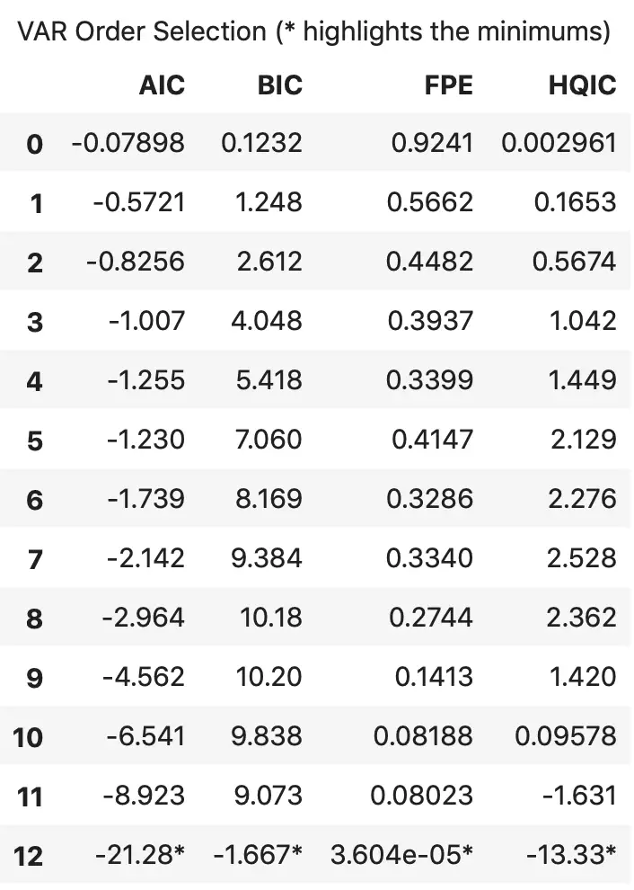
According to FPE and HQIC, the optimal lag is observed at a lag order of 3.

I, however, don’t have an explanation for why the observed AIC and BIC values differ when using result.aic versus as seen using model.select_order().

Since the explicitly computed AIC is the lowest at lag 4, I choose the selected order as 4.

11. Train the VAR Model of Selected Order(p)

model_fitted = model.fit(4)
model_fitted.summary()

Results:

  Summary of Regression Results   
==================================
Model:                         VAR
Method:                        OLS
Date:           Sat, 18, May, 2019
Time:                     11:35:15
--------------------------------------------------------------------
No. of Equations:         8.00000    BIC:                    4.37122
Nobs:                     113.000    HQIC:                  0.584936
Log likelihood:          -905.679    FPE:                   0.155570
AIC:                     -2.00074    Det(Omega_mle):       0.0200322
--------------------------------------------------------------------
Results for equation rgnp
===========================================================================
              coefficient       std. error           t-stat            prob
---------------------------------------------------------------------------
const            2.430021         2.677505            0.908           0.364
L1.rgnp         -0.750066         0.159023           -4.717           0.000
L1.pgnp         -0.095621         4.938865           -0.019           0.985
L1.ulc          -6.213996         4.637452           -1.340           0.180
L1.gdfco        -7.414768        10.184884           -0.728           0.467
L1.gdf         -24.864063        20.071245           -1.239           0.215
L1.gdfim         1.082913         4.309034            0.251           0.802
L1.gdfcf        16.327252         5.892522            2.771           0.006
L1.gdfce         0.910522         2.476361            0.368           0.713
L2.rgnp         -0.568178         0.163971           -3.465           0.001
L2.pgnp         -1.156201         4.931931           -0.234           0.815
L2.ulc         -11.157111         5.381825           -2.073           0.038
L2.gdfco         3.012518        12.928317            0.233           0.816
L2.gdf         -18.143523        24.090598           -0.753           0.451
L2.gdfim        -4.438115         4.410654           -1.006           0.314
L2.gdfcf        13.468228         7.279772            1.850           0.064
L2.gdfce         5.130419         2.805310            1.829           0.067
L3.rgnp         -0.514985         0.152724           -3.372           0.001
L3.pgnp        -11.483607         5.392037           -2.130           0.033
L3.ulc         -14.195308         5.188718           -2.736           0.006
L3.gdfco       -10.154967        13.105508           -0.775           0.438
L3.gdf         -15.438858        21.610822           -0.714           0.475
L3.gdfim        -6.405290         4.292790           -1.492           0.136
L3.gdfcf         9.217402         7.081652            1.302           0.193
L3.gdfce         5.279941         2.833925            1.863           0.062
L4.rgnp         -0.166878         0.138786           -1.202           0.229
L4.pgnp          5.329900         5.795837            0.920           0.358
L4.ulc          -4.834548         5.259608           -0.919           0.358
L4.gdfco        10.841602        10.526530            1.030           0.303
L4.gdf         -17.651510        18.746673           -0.942           0.346
L4.gdfim        -1.971233         4.029415           -0.489           0.625
L4.gdfcf         0.617824         5.842684            0.106           0.916
L4.gdfce        -2.977187         2.594251           -1.148           0.251
===========================================================================

Results for equation pgnp
===========================================================================
              coefficient       std. error           t-stat            prob
---------------------------------------------------------------------------
const            0.094556         0.063491            1.489           0.136
L1.rgnp         -0.004231         0.003771           -1.122           0.262
L1.pgnp          0.082204         0.117114            0.702           0.483
L1.ulc          -0.097769         0.109966           -0.889           0.374

(... TRUNCATED because of long output....)
(... TRUNCATED because of long output....)
(... TRUNCATED because of long output....)

Correlation matrix of residuals
             rgnp      pgnp       ulc     gdfco       gdf     gdfim     gdfcf     gdfce
rgnp     1.000000  0.248342 -0.668492 -0.160133 -0.047777  0.084925  0.009962  0.205557
pgnp     0.248342  1.000000 -0.148392 -0.167766 -0.134896  0.007830 -0.169435  0.032134
ulc     -0.668492 -0.148392  1.000000  0.268127  0.327761  0.171497  0.135410 -0.026037
gdfco   -0.160133 -0.167766  0.268127  1.000000  0.303563  0.232997 -0.035042  0.184834
gdf     -0.047777 -0.134896  0.327761  0.303563  1.000000  0.196670  0.446012  0.309277
gdfim    0.084925  0.007830  0.171497  0.232997  0.196670  1.000000 -0.089852  0.707809
gdfcf    0.009962 -0.169435  0.135410 -0.035042  0.446012 -0.089852  1.000000 -0.197099
gdfce    0.205557  0.032134 -0.026037  0.184834  0.309277  0.707809 -0.197099  1.000000

12. Check for Serial Correlation of Residuals (Errors) using Durbin Watson Statistic

Serial correlation of residuals is used to check if there is any leftover pattern in the residuals (errors).

What does this mean to us?

If there is any correlation left in the residuals, then, there is some pattern in the time series that is still left to be explained by the model. In that case, the typical course of action is to either increase the order of the model or induce more predictors into the system or look for a different algorithm to model the time series.

So, checking for serial correlation is to ensure that the model is sufficiently able to explain the variances and patterns in the time series.

Alright, coming back to topic.

A common way of checking for serial correlation of errors can be measured using the Durbin Watson’s Statistic.

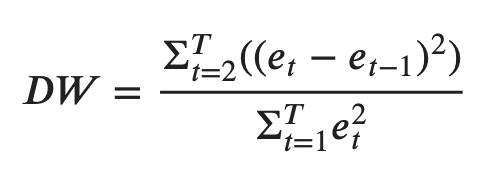
The value of this statistic can vary between 0 and 4. The closer it is to the value 2, then there is no significant serial correlation. The closer to 0, there is a positive serial correlation, and the closer it is to 4 implies negative serial correlation.

from statsmodels.stats.stattools import durbin_watson
out = durbin_watson(model_fitted.resid)

for col, val in zip(df.columns, out):
    print(adjust(col), ':', round(val, 2))

Results:

rgnp   : 2.09
pgnp   : 2.02
ulc    : 2.17
gdfco  : 2.05
gdf    : 2.25
gdfim  : 1.99
gdfcf  : 2.2
gdfce  : 2.17

The serial correlation seems quite alright. Let’s proceed with the forecast.

13. How to Forecast VAR model using statsmodels

In order to forecast, the VAR model expects up to the lag order number of observations from the past data.

This is because, the terms in the VAR model are essentially the lags of the various time series in the dataset, so you need to provide it as many of the previous values as indicated by the lag order used by the model.

# Get the lag order
lag_order = model_fitted.k_ar
print(lag_order)  #> 4

# Input data for forecasting
forecast_input = df_differenced.values[-lag_order:]
forecast_input

4

array([[ 13.5,   0.1,   1.4,   0.1,   0.1,  -0.1,   0.4,  -2. ],
       [-23.6,   0.2,  -2. ,  -0.5,  -0.1,  -0.2,  -0.3,  -1.2],
       [ -3.3,   0.1,   3.1,   0.5,   0.3,   0.4,   0.9,   2.2],
       [ -3.9,   0.2,  -2.1,  -0.4,   0.2,  -1.5,   0.9,  -0.3]])

Let’s forecast.

# Forecast
fc = model_fitted.forecast(y=forecast_input, steps=nobs)
df_forecast = pd.DataFrame(fc, index=df.index[-nobs:], columns=df.columns + '_2d')
df_forecast

The forecasts are generated but it is on the scale of the training data used by the model. So, to bring it back up to its original scale, you need to de-difference it as many times you had differenced the original input data.

In this case it is two times.

14. Invert the transformation to get the real forecast

def invert_transformation(df_train, df_forecast, second_diff=False):
    """Revert back the differencing to get the forecast to original scale."""
    df_fc = df_forecast.copy()
    columns = df_train.columns
    for col in columns:        
        # Roll back 2nd Diff
        if second_diff:
            df_fc[str(col)+'_1d'] = (df_train[col].iloc[-1]-df_train[col].iloc[-2]) + df_fc[str(col)+'_2d'].cumsum()
        # Roll back 1st Diff
        df_fc[str(col)+'_forecast'] = df_train[col].iloc[-1] + df_fc[str(col)+'_1d'].cumsum()
    return df_fc

df_results = invert_transformation(train, df_forecast, second_diff=True)        
df_results.loc[:, ['rgnp_forecast', 'pgnp_forecast', 'ulc_forecast', 'gdfco_forecast',
                   'gdf_forecast', 'gdfim_forecast', 'gdfcf_forecast', 'gdfce_forecast']]

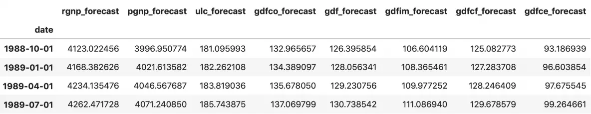
The forecasts are back to the original scale. Let’s plot the forecasts against the actuals from test data.

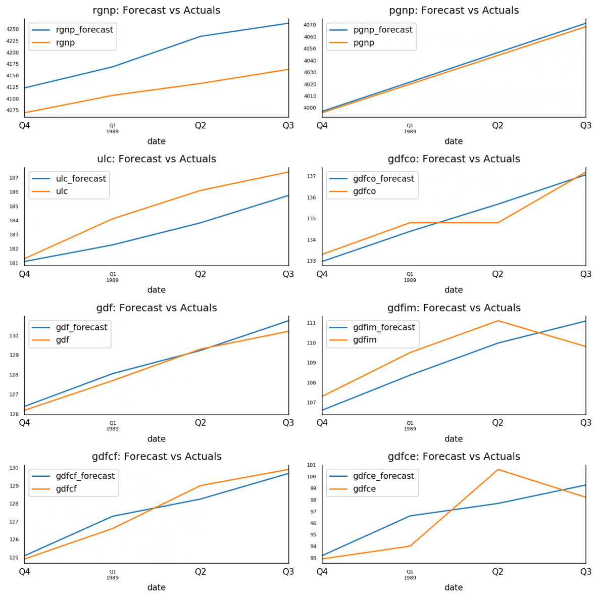
15. Plot of Forecast vs Actuals

fig, axes = plt.subplots(nrows=int(len(df.columns)/2), ncols=2, dpi=150, figsize=(10,10))
for i, (col,ax) in enumerate(zip(df.columns, axes.flatten())):
    df_results[col+'_forecast'].plot(legend=True, ax=ax).autoscale(axis='x',tight=True)
    df_test[col][-nobs:].plot(legend=True, ax=ax);
    ax.set_title(col + ": Forecast vs Actuals")
    ax.xaxis.set_ticks_position('none')
    ax.yaxis.set_ticks_position('none')
    ax.spines["top"].set_alpha(0)
    ax.tick_params(labelsize=6)

plt.tight_layout();

Forecast vs Actuals comparison of VAR model

16. Evaluate the Forecasts

To evaluate the forecasts, let’s compute a comprehensive set of metrics, namely, the MAPE, ME, MAE, MPE, RMSE, corr and minmax.

from statsmodels.tsa.stattools import acf
def forecast_accuracy(forecast, actual):
    mape = np.mean(np.abs(forecast - actual)/np.abs(actual))  # MAPE
    me = np.mean(forecast - actual)             # ME
    mae = np.mean(np.abs(forecast - actual))    # MAE
    mpe = np.mean((forecast - actual)/actual)   # MPE
    rmse = np.mean((forecast - actual)**2)**.5  # RMSE
    corr = np.corrcoef(forecast, actual)[0,1]   # corr
    mins = np.amin(np.hstack([forecast[:,None], 
                              actual[:,None]]), axis=1)
    maxs = np.amax(np.hstack([forecast[:,None], 
                              actual[:,None]]), axis=1)
    minmax = 1 - np.mean(mins/maxs)             # minmax
    return({'mape':mape, 'me':me, 'mae': mae, 
            'mpe': mpe, 'rmse':rmse, 'corr':corr, 'minmax':minmax})

print('Forecast Accuracy of: rgnp')
accuracy_prod = forecast_accuracy(df_results['rgnp_forecast'].values, df_test['rgnp'])
for k, v in accuracy_prod.items():
    print(adjust(k), ': ', round(v,4))

print('\nForecast Accuracy of: pgnp')
accuracy_prod = forecast_accuracy(df_results['pgnp_forecast'].values, df_test['pgnp'])
for k, v in accuracy_prod.items():
    print(adjust(k), ': ', round(v,4))

print('\nForecast Accuracy of: ulc')
accuracy_prod = forecast_accuracy(df_results['ulc_forecast'].values, df_test['ulc'])
for k, v in accuracy_prod.items():
    print(adjust(k), ': ', round(v,4))

print('\nForecast Accuracy of: gdfco')
accuracy_prod = forecast_accuracy(df_results['gdfco_forecast'].values, df_test['gdfco'])
for k, v in accuracy_prod.items():
    print(adjust(k), ': ', round(v,4))

print('\nForecast Accuracy of: gdf')
accuracy_prod = forecast_accuracy(df_results['gdf_forecast'].values, df_test['gdf'])
for k, v in accuracy_prod.items():
    print(adjust(k), ': ', round(v,4))

print('\nForecast Accuracy of: gdfim')
accuracy_prod = forecast_accuracy(df_results['gdfim_forecast'].values, df_test['gdfim'])
for k, v in accuracy_prod.items():
    print(adjust(k), ': ', round(v,4))

print('\nForecast Accuracy of: gdfcf')
accuracy_prod = forecast_accuracy(df_results['gdfcf_forecast'].values, df_test['gdfcf'])
for k, v in accuracy_prod.items():
    print(adjust(k), ': ', round(v,4))

print('\nForecast Accuracy of: gdfce')
accuracy_prod = forecast_accuracy(df_results['gdfce_forecast'].values, df_test['gdfce'])
for k, v in accuracy_prod.items():
    print(adjust(k), ': ', round(v,4))

Forecast Accuracy of: rgnp
mape   :  0.0192
me     :  79.1031
mae    :  79.1031
mpe    :  0.0192
rmse   :  82.0245
corr   :  0.9849
minmax :  0.0188

Forecast Accuracy of: pgnp
mape   :  0.0005
me     :  2.0432
mae    :  2.0432
mpe    :  0.0005
rmse   :  2.146
corr   :  1.0
minmax :  0.0005

Forecast Accuracy of: ulc
mape   :  0.0081
me     :  -1.4947
mae    :  1.4947
mpe    :  -0.0081
rmse   :  1.6856
corr   :  0.963
minmax :  0.0081

Forecast Accuracy of: gdfco
mape   :  0.0033
me     :  0.0007
mae    :  0.4384
mpe    :  0.0
rmse   :  0.5169
corr   :  0.9407
minmax :  0.0032

Forecast Accuracy of: gdf
mape   :  0.0023
me     :  0.2554
mae    :  0.29
mpe    :  0.002
rmse   :  0.3392
corr   :  0.9905
minmax :  0.0022

Forecast Accuracy of: gdfim
mape   :  0.0097
me     :  -0.4166
mae    :  1.06
mpe    :  -0.0038
rmse   :  1.0826
corr   :  0.807
minmax :  0.0096

Forecast Accuracy of: gdfcf
mape   :  0.0036
me     :  -0.0271
mae    :  0.4604
mpe    :  -0.0002
rmse   :  0.5286
corr   :  0.9713
minmax :  0.0036

Forecast Accuracy of: gdfce
mape   :  0.0177
me     :  0.2577
mae    :  1.72
mpe    :  0.0031
rmse   :  2.034
corr   :  0.764
minmax :  0.0175

17. Conclusion

In this article we covered VAR from scratch beginning from the intuition behind it, interpreting the formula, causality tests, finding the optimal order of the VAR model, preparing the data for forecasting, build the model, checking for serial autocorrelation, inverting the transform to get the actual forecasts, plotting the results and computing the accuracy metrics.

Hope you enjoyed reading this as much as I did writing it. I will see you in the next one.

Time Series

Granger Causality Test in Python

Aug 30, 2022

Time Series

Granger Causality Test

Aug 29, 2022

Time Series

ARIMA Model – Complete Guide to Time Series Forecasting in Python

Aug 22, 2021

Time Series

Augmented Dickey Fuller Test (ADF Test) – Must Read Guide

Nov 02, 2019

Time Series

KPSS Test for Stationarity

Time Series