


Confidence interval is a measure to quantify the uncertainty in an estimated statistic (like the mean) when the true population parameter is unknown.
 Training Custom Text Classification Model in spaCy. Photo by Jessica Wong.
You will know
1. What is Confidence Interval?
2. Two types of Confidence Intervals problems
3. Difference between Population parameter vs Sample statistic
4. Confidence Interval Formula
5. Example 1: Estimating Confidence Interval when population standard deviation is not known
6. Example 2: Estimating Confidence Interval when the population standard deviation is known
7. Confidence interval of a proportion”>7. Confidence interval of a proportion
8. Bootstrapping in Statistics: How to Compute Confidence Interval with Bootstrapping
1. What is Confidence Interval?
Confidence interval is a measure to quantify the uncertainty in an estimated statistic (like mean of a certain quantity) when the true population parameter is unknown.
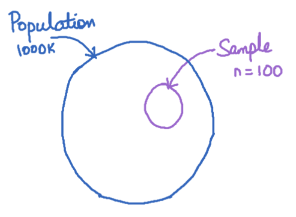
The reason I specifically mention the term ‘population parameter’ is because, usually when you deal with data, you will have data of a smaller sample from the population. While you can easily compute a sample statistic (example: average weight of sample of 10 adult mice), the true population parameter (example: average weight of ALL adult mice that exists) is usually unknown (not always).
In simpler terms, confidence interval provides the upper and lower bounds between which a given estimated statistic can vary. This range between which the statistic can vary is usually referred to as the ‘margin of error’.
Let’s understand with an example
Let’s suppose you want to know the expected annual yield for a given variety of Palm tree in a given region. To know this, you start collecting annual yield data from a small sample of trees. Based on this sample data you want to know the expected yield of that variety ‘in general’ and what could be the range of values the annual yield can take assuming a 95% certainty (confidence).
Understanding confidence intervals can help you answer that question.
However, this is just one example. There can be multiple flavors of ‘confidence intervals problems’. In this post, you will encounter such problems.
Also remember, when someone refers to confidence levels of a given statistic, it it is usually the 95% confidence level by default. As you increase the confidence level further, the margin of error (that is the confidence interval band) become wider.
2. Two types of Confidence Intervals problems
When you speak of confidence intervals, there are largely two types of problems where you would compute confidence intervals. The formula to compute confidence interval changes depending on the type.
- Confidence interval of a sample.
Example: Find the confidence interval for mean weight of adult white mice. - Confidence interval of a proportion.
Example: Find the confidence interval of the percentage of voters who voted for candidate A in an election (based only on exit polls data).
Depending on the type of problem, you need to apply the appropriate formula to calculate confidence intervals.
Secondly, the approach you take to compute the confidence intervals depends on what information you know about the population.

For example, in most real world cases, you would only be working with a small sample and not know anything about the population, particularly it’s standard deviation. If that is the case, you will use the T-distribution approach. However, sometimes, you may know the population standard deviation, in which case you will use the Standard normal distribution based approach.
If this doesn’t make sense to you yet, that’s ok, because all of it will be explained. But you need to first understand the difference between a ‘Population parameter’ vs a ‘Sample statistic’.
3. Difference between Population parameter vs Sample statistic
Well as the name suggests, a population parameter (like mean, standard deviation, etc) is one which is computed or known from the entire population. Whereas, a sample statistic is computed from a smaller sample from the entire population.
The population parameter is hard to get/compute. Otherwise we would not be bothering so much about statistics. Besides, this is where confidence intervals come into picture. Since it is often not practical to compute the population parameter, we compute the statistic from a smaller sample and then estimate a confidence interval between which the true population parameter may vary.
This post is all about computing the confidence intervals in various situations in detail.
A classic example of this is during presidential / parliamentary elections. Here, the entire pool of voters in a country forms the population. And once the election is complete, you may see exit polls results (flashing on TV/Internet) showing a certain confidence interval percentage for the victory of a certain candidate. These exit polls are in fact conducted only on a smaller samples of voters. So, it is considered as a sample statistic upon which the confidence intervals of chance of winning for a given candidate is estimated. By the way, elections are one of the rare occasions where the population parameter itself is actually estimated.
You may have noticed that exit polls conducted in unbiased way often tend to predict the winning candidate correctly.
Exceptions do happen in cases where there is a bias in the sampling approach or when there is a strong overlap between the confidence intervals of candidates.
4. Confidence Interval Formula
The formula and method of estimating confidence interval depends on whether the population’s standard deviation is known on not.
If population standard deviation is known, then:
$$ Confidence \; Interval = \bar{X} \pm Z_{crit}\frac{\sigma}{\sqrt{n}} $$
If population standard deviation is not known, then:
$$ Confidence \; Interval = \bar{X} \pm T_{crit}\frac{s}{\sqrt{n}} $$
Where,
- x̄ is the mean value of observations,
- Z_crit is the critical value of Z-score for the respective confidence level from Standard Normal distribution
- T_crit is the critical value of Z-score for the respective confidence level from T-distribution
- s is the standard deviation of the sample
- σ is the standard deviation of the population
- n is the number of observations in the sample.
The main difference in the calculation is, you have to look up the Z table when the population standard deviation is known. Else, look up the T-distribution table.
5. Example 1: Estimating Confidence Interval when population standard deviation is not known
This is the most common case. Let’s try to understand this with a simple (and nearly stupid) example.
Let’s suppose you want to know the mean height of all male humans on planet earth. It’s not practical to get measurements of the heights of all the humans at a given time. Maybe in today’s world it might be possible with a superhuman effort, but you know what I mean.
So, instead of setting out on such an impractical task, you might rather be content to know a certain mean height computed from a smaller sample and know with a certain confidence how far away it may be from the actual mean height, so you get a sense of what the ‘true mean height’ of the entire population could be.
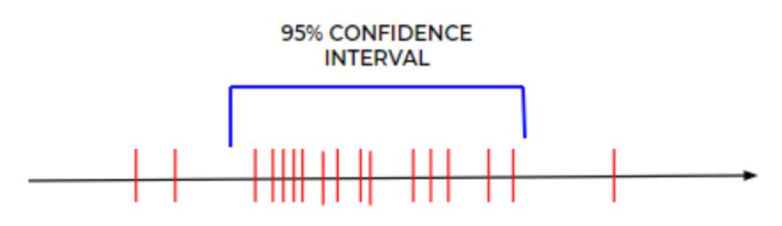
Also, Generally when you see the term confidence interval, it generally refers to 95% confidence interval. That means, the true mean occurs in this given range with 0.95 probability. Some of the other confidence levels frequently used are 90%, 99%, 99.5% confidence interval, which refers to 0.9, 0.99, 0.995 probability respectively. This probability corresponds to the area under the sampling distribution (typically a T-Distribution or a Standard Normal Distribution) that covers as much proportion.
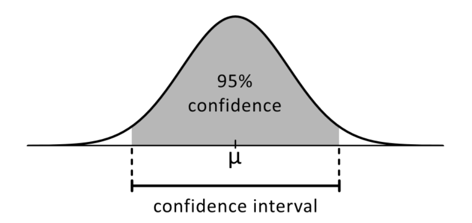
The middle part in the graph(white) represents the 95% confidence interval. It means, if you take any sample of heights from humans (from above example), then there is a 95% chance that it lies inside the white region. The other 2 parts represents the rest 5% chance.
For this example, let’s take a sample data set containing 5 observations of heights: – 160, 165, 170, 175, 180.
All you need to estimate the confidence interval of the mean can be directly computed, except for the Z value, for which you may look up the T-table.
The following information is computed:
- The mean of the sample: 170.
- The standard deviation of sample: 7.071.
- n = 5
For this example, we don’t know the standard deviation of the population. So, you will use the formula that uses the t-critcal value as T-distribution is appropriate for small samples.
$$Confidence \; Interval = \bar{X} \pm T_{crit}\frac{s}{\sqrt{n}} $$
The only item missing is the T-critical value.
So look up the T-Table for degree of freedom = 5-1 = 4 and alpha = (1-0.95)/2 = 0.025.
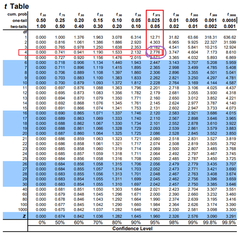
Substituting in formula, you get:
Confidence Intervals = {170 – 2.776 (7.071/sqrt(5)), 170 + 2.776 (7.071/sqrt(5))}
= {161.221, 178.778}
Exercises:
- What is the 99% Confidence Intervals for the same problem?
- How can the problem be changed so you get a narrower range of 99% confidence interval?
6. Example 2: Estimating Confidence Interval when the population standard deviation is known
Problem Statement:
An online management admission test is designed to have a standard deviation of 7.071. Estimate the 95% confidence intervals when there were 5 members in the sample which had a sample mean of 170.
Solution:
Since you have a problem where you know the population standard deviation, use the Z-score based formula to compute the confidence intervals.
$$Confidence \; Interval = \bar{X} \pm Z_{crit}\frac{\sigma}{\sqrt{n}} $$
The following information is known:
The mean of the sample: 170.
The standard deviation of sample: 7.071.
n = 5
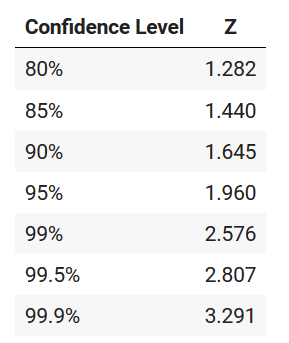
If you want to calculate the 95% confidence interval, then the Z-critical value is 1.96. That means, the total area under the curve for a distance of 1.96 standard deviations from the center of the standard normal distribution on either side is 0.95, where the total area under the curve is taken as 1.0.
Likewise, the critical z-value for various other commonly used confidence levels is shown below:
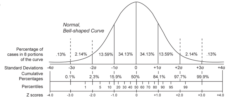
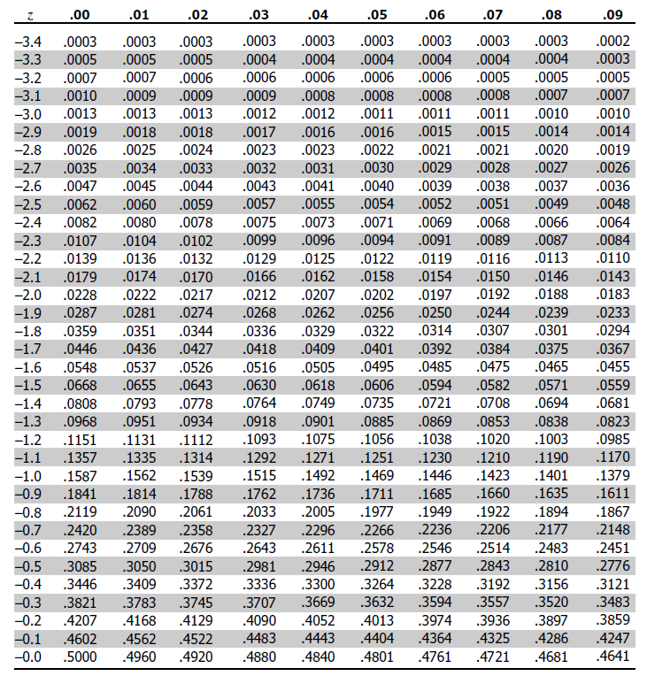
Alternately, you can look up the Z-value from the Z-table below.
How to interpret the z-table?
The values in the table show the area under the standard normal distribution curve that is to the left of ‘z’ standard deviations from the mean.
For 95% confidence level, you want to look for the value of ‘z’ that produces a value of 0.025 when the column value is 0.05. Turns out the Z value you are looking for (left most column) falls between -1.9 to -2.0. -1.96 to be precise, which is not available upto the desired decimals in this table. To make things easier, refer to the table above for the desired z-scores.
Substitute these values in the formula, you will get:
Confidence Intervals = {170 – 1.96 (7.071/sqrt(5)), 70 + 1.96 (7.071/sqrt(5))}
= {163.802, 176.198}
the value to be 170 +/- 6.198, where 6.198 is called as the margin of error.
This means that if you take any range of values from the data set, there is a 95% probability that the value will lie between 163.802 and 176.198.
Since the formula has sqrt(n) in the denominator, the larger the number of samples you have, smaller will be the margin of error and thereby the smaller the confidence interval will be, which also means, more precise the estimate will be.
7. Confidence interval of a proportion
When your sample data is made up of binary values (like 1 vs 0, yes vs no) you are dealing with the problem of proportions.
For example, you might want to find the confidence interval of number of people who voted ‘yes’ in a certain shareholders voting call. In this case, the regular concept of standard deviation does not apply in the sense it does with whole numbered data.
When you want to compute the confidence interval for proportions, you need to use a slightly different formula:
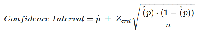
Where, p is the sample’s proportion of interest.
Let’s look at a simple example.
Problem Statement
Two candidates A and B are contesting in an election. Out of the total 10000 people participating in an election, 100 were randomly surveyed at exit polls. Of that 27 voted for candidate A.
Find the 99% confidence interval of the true proportion of people who voted for candidate A.
Solution:
Here is what we know:
N = 10000
n = 100
p = 27/100 = 0.27
1-p = 1-0.27 = 0.73
Since you want 99% CI, Z-critical = 2.576
Substituting all the values in the formula gives:
Confidence Interval = {0.27 + [2.576 sqrt(0.27 0.73 / 100)], 0.27 – [2.576 sqrt(0.27 0.73 / 100)]}
= {0.3843, 0.1556}
8. Bootstrapping in Statistics: How to Compute Confidence Interval with Bootstrapping
First, What does ‘bootstrapping’ mean in statistics?
Bootstrapping is a sampling technique where you repeatedly sample same number of observations in the data but with replacement. And you do this for a large number of iterations (say 1000 or more).
By doing this you will get a large number of simulated datasets where, in each data set, you will have some observations repeated. Because, the random sampling is done ‘with replacement’.
Now, In each of the simulated samples you compute the statistic, like the ‘mean’ in this case, and note it down for a large number of observations.
Let’s say, you computed the mean of the heights for the above example this way. You might expect the mean computed from each of the simulated samples to be slightly different (as shown below).
Now, how to calculate the confidence intervals?
The 95% confidence interval of the mean is nothing but the interval that covers 95% of these data points.
Bootstrapping is purely a sampling based technique, it can be used to estimate the confidence intervals regardless of what distribution your data follows.
For sake of clarity, let’s write down the steps to calculate the confidence interval:
Step 1: Randomly sample as many items in the dataset with replacement.
Step 2: Calculate the mean (or whatever statistic) of that sample.
Step 3: Repeat Step 1 and 2 for a large number of iterations and plot them in a graph if you want to visualize. The 95% confidence interval is the range that covers 95% of the simulated means.
Anything outside that 95% interval, has lower probability of occurring.
Hope you have a fair idea about confidence interval now? Leave your thoughts in the comments below. More such posts are in the works, subscribe to my mailing list to hear from me.

