System of Equations – Understanding Linear Algebra System of Equations and Plotting

Linear algebra, often considered the cornerstone of advanced mathematics and foundational to multiple scientific fields, is primarily concerned with vector spaces and linear equations. One of its most fundamental concepts is the system of linear equations. Let’s delve into this topic to understand its significance and intricacies.

What is a System of Linear Equations?

At its core, a system of linear equations is a collection of two or more linear equations with common variables. If you’ve ever encountered problems where you had to find the intersection point of two lines, you’ve effectively worked with a system of two linear equations.

For instance:

1. x + y = 5

2. 2x − 3y = 12

These are two linear equations with two variables, x and y.

Methods of Solving

Several methods can solve a system of linear equations:

1. Graphical Method: Plot each equation on a graph and identify the point(s) of intersection.

2. Substitution Method: Express one variable in terms of the other from one equation and substitute this expression in the other equation.

3. Elimination Method: Add or subtract the equations to eliminate one variable, making it easier to solve for the other.

4. Matrix Method: Utilize the properties of matrices to solve the system.

The Concept of Determinants

In the context of a system of linear equations with two variables, the determinant can be thought of as the area scaling factor of a transformation. If the determinant of the coefficient matrix (A) is zero, it implies that the rows (equations) are linearly dependent, and the system doesn’t have a unique solution.

For our example:
Determinant of A = 1(−1)−1(2)=−3, which is not zero. Therefore, our system has a unique solution.

Unique Solution, No Solution, or Infinite Solutions?

The nature of the solution of a system depends on the determinant and the nature of the equations:

1. Unique Solution: The lines represented by the equations intersect at a single point.
2. No Solution: The lines are parallel and never intersect.
3. Infinite Solutions: The equations represent the same line.

The determinant of a matrix

A is often denoted as det(A) or ∣ A∣.

For a 2×2 matrix:

$If = \begin{bmatrix}
a & b \\
c & d \\
\end{bmatrix}$

then its determinant is given by det(A) = ad − bc.

For a 3×3 matrix:

$If = \begin{bmatrix}
a & b & c \\
d & e & f \\
g & h & i \\
\end{bmatrix}$

then its determinant is: det(A) = aei + bfg + cdh − ceg − afh − bdi.

Representing Equations in Matrix Form

x + y = 5

2x − 3y = 12

The above system can be represented in matrix form as:

A⋅X = B

Where,

$
\begin{bmatrix}
1 & 1 \\
2 & 3 \\
\end{bmatrix}$

$ \begin{bmatrix}
x \\
y \\
\end{bmatrix}$

$
\begin{bmatrix}
5 \\
12 \\
\end{bmatrix}$

Plotting System of Equations

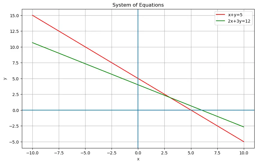
To visualize the system of equations, we can plot each equation on a 2D graph.

Using Python’s matplotlib and numpy libraries, let’s plot the given system:

import numpy as np
import matplotlib.pyplot as plt

x = np.linspace(-10, 10, 400)

# Given the equation: x + y = 5
# y = 5 - x
y1 = 5 - x

# Given the equation: 2x + 3y = 12
# y = (12 - 2x) / 3
y2 = (12 - 2*x) / 3

plt.figure(figsize=(10,6))
plt.plot(x, y1, '-r', label='x+y=5')
plt.plot(x, y2, '-g', label='2x+3y=12')
plt.title('System of Equations')
plt.xlabel('x', color='#1C2833')
plt.ylabel('y', color='#1C2833')
plt.legend(loc='upper right')
plt.grid()
plt.axhline()
plt.axvline()
plt.show()

This code will plot the two equations. The intersection point is the solution to the system.

Solving the System using Python

Python’s numpy library can be used to solve this system:

A = np.array([[1, 1], [2, 3]])
B = np.array([5, 12])

# Using numpy's linear algebra solver
X = np.linalg.solve(A, B)
print(X)  # Output: [x-value, y-value]

[3. 2.]

Gaussian Elimination and LU Decomposition

When solving systems of linear equations, one of the classic methods is the Gaussian elimination. It involves converting a system of linear equations into an upper triangular matrix form, then using back substitution to find the variables. LU Decomposition breaks down matrix A into the product of a lower triangular matrix L and an upper triangular matrix U.

Here’s how you can solve the system of equations using LU decomposition in Python:

import numpy as np
import scipy.linalg

A = np.array([[1, 1], [2, 3]])
B = np.array([5, 12])

# Perform LU decomposition
P, L, U = scipy.linalg.lu(A)

# Forward substitution to solve Ly = B
y = np.linalg.solve(L, P @ B)

# Back substitution to solve Ux = y
X = np.linalg.solve(U, y)
print(X)  # Output: [x-value, y-value]

[3. 2.]

Matrix Inversion

Another method to solve a system of linear equations is by using the inverse of a matrix. However, keep in mind that not all matrices are invertible, and this method can be computationally expensive for large matrices.

For the system

A ⋅ X = B,

If matrix

A is invertible, then

X = A −1 ⋅ B.

Python code to find X using matrix inversion:

# Calculate the inverse of A
A_inv = np.linalg.inv(A)

# Multiply A_inv with B to get X
X = np.dot(A_inv, B)
print(X)  # Output: [x-value, y-value]

[3. 2.]

Wrapping Up

Linear algebra’s systems of equations form the bedrock for numerous mathematical, physical, and engineering problems. Python, with its rich ecosystem of libraries, serves as an incredible tool to visualize, interpret, and solve these systems.

As you delve deeper, you’ll unravel more intricate relationships and methods, bridging abstract mathematical concepts with tangible real-world applications.