

Probability and statistics are often viewed as complex areas of study. However, by using real-world examples and some visual aids, the seemingly challenging concepts become quite intuitive. Let’s deep dive into discrete frequency distributions and the different types of Probability Mass Functions (PMFs).

In this Blog post we will learn:
- Discrete Frequency Distribution:
- Types of Discrete Frequency Distribution:
2.1. Simple Frequency Distribution:
2.2. Grouped Frequency Distribution:
2.3. Cumulative Frequency Distribution: - Probability Mass Function (PMF):
- Types of Probability Mass Functions (PMFs):
4.1. Bernoulli PMF:
4.2. Binomial PMF:
4.3. Poisson PMF: - Wrapping Up
1. Discrete Frequency Distribution:
When data is collected and organized in a systematic manner, it’s often represented in a frequency distribution. If the data is discrete, which means it consists of distinct or separate values, then we can represent it using a Discrete Frequency Distribution.
Example: Imagine we did a survey in a classroom of 30 students asking them how many siblings they have. The results might look something like:
| Number of Siblings | Frequency |
|---|---|
| 0 | 5 |
| 1 | 10 |
| 2 | 8 |
| 3 | 5 |
| 4 | 2 |
From this table, we can deduce that 5 students have no siblings, 10 have one sibling, 8 have two siblings, and so on. This is a Discrete Frequency Distribution because we are looking at distinct numbers of siblings.
2. Types of Discrete Frequency Distribution:
Before jumping into PMFs, let’s first understand discrete frequency distributions. It’s simply a summary of data occurrence in a table that shows the frequency of different outcomes.
2.1. Simple Frequency Distribution:
Scenario: Imagine working in an office. During a casual survey, you ask your colleagues about their daily coffee consumption.
| Cups of Coffee | Number of Employees |
|---|---|
| 0 | 5 |
| 1 | 8 |
| 2 | 6 |
| 3 | 4 |
This table tells you that 5 employees don’t drink coffee, 8 drink just one cup, and so on.
2.2. Grouped Frequency Distribution:
Scenario: Think of a bookstore. They record the number of books purchased by each customer during a sale.
| Number of Books (Grouped) | Number of Customers |
|---|---|
| 1 – 5 | 20 |
| 6 – 10 | 15 |
| 11 – 15 | 10 |
| 16 – 20 | 5 |
This representation groups the data, so you know 20 customers bought between 1 to 5 books, 15 customers bought 6 to 10 books, and so forth.
2.3. Cumulative Frequency Distribution:
Using the bookstore example above, let’s determine the cumulative number of customers who bought up to a certain number of books.
| Number of Books (Grouped) | Cumulative Number of Customers |
|---|---|
| Up to 5 | 20 |
| Up to 10 | 35 (20+15) |
| Up to 15 | 45 (20+15+10) |
| Up to 20 | 50 (20+15+10+5) |
This table reveals the total number of customers who bought a certain number of books or fewer.
3. Probability Mass Function (PMF):
For a discrete random variable, the probability that the variable takes a specific value is given by a function, which is called the Probability Mass Function (PMF). In simpler terms, PMF gives us the probability of each possible outcome of a discrete random variable.
To find the PMF from a discrete frequency distribution, we’ll divide each frequency by the total number of observations (or sample size).

Continuing our example: If we want to find out the probability of randomly selecting a student from the class who has a specific number of siblings, we’d compute the PMF.
| Number of Siblings | Frequency | Probability (PMF) |
|---|---|---|
| 0 | 5 | 5/30 = 0.1667 |
| 1 | 10 | 10/30 = 0.3333 |
| 2 | 8 | 8/30 = 0.2667 |
| 3 | 5 | 5/30 = 0.1667 |
| 4 | 2 | 2/30 = 0.0667 |
4. Types of Probability Mass Functions (PMFs):
Having understood discrete frequency distributions, let’s journey into PMFs. For discrete random variables, PMFs give the probability of specific outcomes.
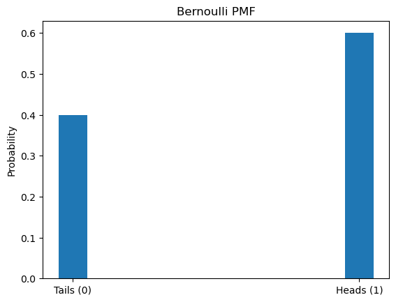
4.1. Bernoulli PMF:
Scenario: Coin flipping – the classic probability example. With each flip, you can get Heads (1) or Tails (0).
Sample Flips: 0, 1, 0, 0, 1, 1, 0, 1, 1, 1
For this, the Bernoulli PMF is: $P(X=k) = p^k(1-p)^{1-k}$
Where:
– $p$ is the probability of Heads.
– $k$ can be either 0 (Tails) or 1 (Heads).
import matplotlib.pyplot as plt
import numpy as np

data = [0, 1, 0, 0, 1, 1, 0, 1, 1, 1]
p = sum(data) / len(data)

def bernoulli_pmf(k):
    return p**k * (1-p)**(1-k)

values = [0, 1]
probabilities = [bernoulli_pmf(k) for k in values]

plt.bar(values, probabilities, width=0.1)
plt.xticks(values, ['Tails (0)', 'Heads (1)'])
plt.ylabel('Probability')
plt.title('Bernoulli PMF')
plt.show()
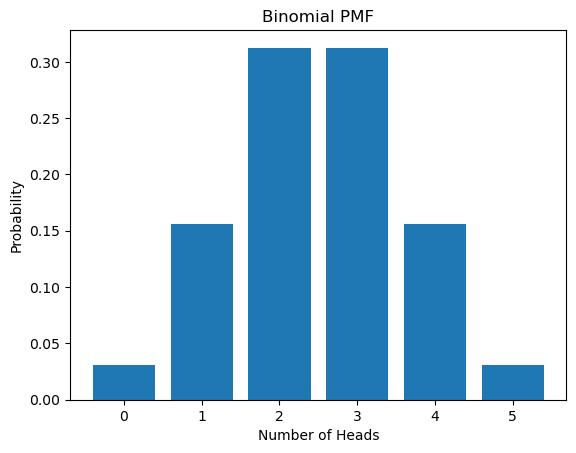
4.2. Binomial PMF:
This represents the number of successes in a fixed number of trials with the same probability of success.
Scenario: Let’s remain with our coin. Now, flip it five times. How likely is it to get any number of heads between 0 and 5?
For this, the Binomial PMF is: $P(X=k) = \binom{n}{k} p^k(1-p)^{n-k}$
Where:
– $n$ is the number of flips.
– $p$ is the probability of a head.
– $k$ is the number of heads.
from scipy.stats import binom

n = 5
p = 0.5
k_values = np.arange(0, n+1)
probabilities = binom.pmf(k_values, n, p)

plt.bar(k_values, probabilities)
plt.xlabel('Number of Heads')
plt.ylabel('Probability')
plt.title('Binomial PMF')
plt.show()
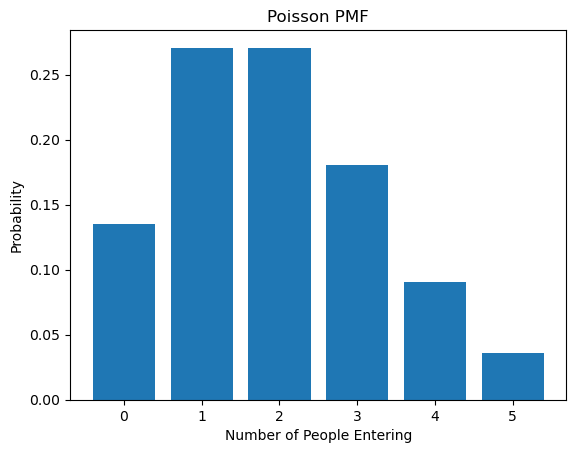
4.3. Poisson PMF:
This describes the probability of observing a given number of events in a fixed interval of time or space. The events must occur with a known constant mean rate and be independent of the time since the last event
Scenario: A librarian counts how many people enter the library every 10 minutes. On average, it’s 2 people. So, what’s the likelihood of a given number of people entering in any 10-minute window?
The Poisson PMF is: $P(X=k) = \frac{\lambda^k e^{-\lambda}}{k!}$
Where:
– $\lambda$ is the average rate (2 people every 10 minutes).
– $k$ is the number of people.
from scipy.stats import poisson

lambda_val = 2
k_values = np.arange(0, 6)
probabilities = poisson.pmf(k_values, lambda_val)

plt.bar(k_values, probabilities)
plt.xlabel('Number of People Entering')
plt.ylabel('Probability')
plt.title('Poisson PMF')
plt.show()
5. Wrapping Up
From understanding our colleagues’ coffee habits to predicting how many people enter a library, the tools of discrete frequency distributions and PMFs offer powerful insights into everyday events. With Python, these abstract concepts not only become comprehensible but also visually appealing.

