PySpark Mllib K-Means Clustering – Mastering K-means Clustering with PySpark MLlib and Example Code

Lets explore K-means clustering using PySpark’s MLlib library in-depth. PySpark is an open-source Python library that facilitates distributed data processing and offers a simple way to run machine learning algorithms on large-scale data.

K-means clustering is a widely-used unsupervised machine learning algorithm that partitions a dataset into K distinct clusters based on the features of the data points.

To demonstrate K-means clustering with PySpark MLlib, we will use a sample dataset containing customer data with three features: age, income, and spending score. Our objective is to group the customers into clusters based on these features to understand their behavior and target them with personalized marketing strategies.

1. Import required libraries and initialize SparkSession

First, let’s import the necessary libraries and create a SparkSession, the entry point to use PySpark.

import findspark
findspark.init()
from pyspark import SparkFiles
from pyspark.sql import SparkSession

from pyspark.ml.feature import VectorAssembler, StandardScaler
from pyspark.ml.clustering import KMeans
from pyspark.ml.evaluation import ClusteringEvaluator
import matplotlib.pyplot as plt
import pandas as pd

spark = SparkSession.builder.appName("Mastering K-means Clustering with PySpark MLlib").getOrCreate()

2. Load the dataset

For this example, we will use the Breast Cancer Wisconsin (Diagnostic) dataset

url = "https://raw.githubusercontent.com/selva86/datasets/master/Iris.csv"
spark.sparkContext.addFile(url)

df = spark.read.csv(SparkFiles.get("Iris.csv"), header=True, inferSchema=True)
df.show(5)

+---+-------------+------------+-------------+------------+-----------+
| Id|SepalLengthCm|SepalWidthCm|PetalLengthCm|PetalWidthCm|    Species|
+---+-------------+------------+-------------+------------+-----------+
|  1|          5.1|         3.5|          1.4|         0.2|Iris-setosa|
|  2|          4.9|         3.0|          1.4|         0.2|Iris-setosa|
|  3|          4.7|         3.2|          1.3|         0.2|Iris-setosa|
|  4|          4.6|         3.1|          1.5|         0.2|Iris-setosa|
|  5|          5.0|         3.6|          1.4|         0.2|Iris-setosa|
+---+-------------+------------+-------------+------------+-----------+
only showing top 5 rows

3. Data Preprocessing

Before performing K-means clustering, preprocess the data by assembling the features into a single column and scaling the features to a comparable range

# Assembling features into a single column
assembler = VectorAssembler(inputCols=["SepalLengthCm", "SepalWidthCm", "PetalLengthCm", "PetalWidthCm"], outputCol="features")
data_df = assembler.transform(df)

# Scaling the features
scaler = StandardScaler(inputCol="features", outputCol="scaled_features")
scaler_model = scaler.fit(data_df)
data_df = scaler_model.transform(data_df)

data_df.show(5)

+---+-------------+------------+-------------+------------+-----------+-----------------+--------------------+
| Id|SepalLengthCm|SepalWidthCm|PetalLengthCm|PetalWidthCm|    Species|         features|     scaled_features|
+---+-------------+------------+-------------+------------+-----------+-----------------+--------------------+
|  1|          5.1|         3.5|          1.4|         0.2|Iris-setosa|[5.1,3.5,1.4,0.2]|[6.15892840883878...|
|  2|          4.9|         3.0|          1.4|         0.2|Iris-setosa|[4.9,3.0,1.4,0.2]|[5.9174018045706,...|
|  3|          4.7|         3.2|          1.3|         0.2|Iris-setosa|[4.7,3.2,1.3,0.2]|[5.67587520030241...|
|  4|          4.6|         3.1|          1.5|         0.2|Iris-setosa|[4.6,3.1,1.5,0.2]|[5.55511189816831...|
|  5|          5.0|         3.6|          1.4|         0.2|Iris-setosa|[5.0,3.6,1.4,0.2]|[6.03816510670469...|
+---+-------------+------------+-------------+------------+-----------+-----------------+--------------------+
only showing top 5 rows

4. Finding the Optimal Number of Clusters (K)

One of the challenges with K-means clustering is determining the optimal number of clusters (K). We can use the “elbow method” to find the best K value by plotting the Within Set Sum of Squared Errors (WSSSE) for different K values and finding the “elbow point”

# Computing WSSSE for K values from 2 to 8
wssse_values =[]
evaluator = ClusteringEvaluator(predictionCol='prediction', featuresCol='scaled_features', \
                                metricName='silhouette', distanceMeasure='squaredEuclidean')

for i in range(2,8):    
    KMeans_mod = KMeans(featuresCol='scaled_features', k=i)  
    KMeans_fit = KMeans_mod.fit(data_df)  
    output = KMeans_fit.transform(data_df)   
    score = evaluator.evaluate(output)   
    wssse_values.append(score)  
    print("Silhouette Score:",score)

Silhouette Score: 0.7714149126311811
Silhouette Score: 0.673053224228898
Silhouette Score: 0.5828460108251851
Silhouette Score: 0.5177329198703228
Silhouette Score: 0.5315277151877008
Silhouette Score: 0.5308094572223238

# Plotting WSSSE values
plt.plot(range(1, 7), wssse_values)
plt.xlabel('Number of Clusters (K)')
plt.ylabel('Within Set Sum of Squared Errors (WSSSE)')
plt.title('Elbow Method for Optimal K')
plt.grid()
plt.show()

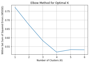
From the plot, we can observe an “elbow point” where the decrease in WSSSE slows down. In our example, let’s assume that the optimal K value is 4.

5. Performing K-means Clustering

With the preprocessed data and the optimal K value, we can perform K-means clustering using the KMeans class from the PySpark MLlib library

# Define the K-means clustering model
kmeans = KMeans(k=4, featuresCol="scaled_features", predictionCol="cluster")
kmeans_model = kmeans.fit(data_df)

# Assigning the data points to clusters
clustered_data = kmeans_model.transform(data_df)

6. Evaluating the Model

To evaluate the quality of the clustering, we can use the Within Set Sum of Squared Errors (WSSSE) metric

output = KMeans_fit.transform(data_df)
wssse = evaluator.evaluate(output)
print(f"Within Set Sum of Squared Errors (WSSSE) = {wssse}")

Within Set Sum of Squared Errors (WSSSE) = 0.5308094572223238

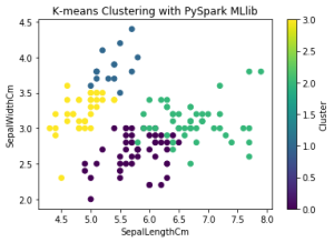
7. Visualizing the Results

Finally, let’s convert the clustered data to a Pandas DataFrame and visualize the results using a scatter plot

# Converting to Pandas DataFrame
clustered_data_pd = clustered_data.toPandas()

# Visualizing the results
plt.scatter(clustered_data_pd["SepalLengthCm"], clustered_data_pd["SepalWidthCm"], c=clustered_data_pd["cluster"], cmap='viridis')
plt.xlabel("SepalLengthCm")
plt.ylabel("SepalWidthCm")
plt.title("K-means Clustering with PySpark MLlib")
plt.colorbar().set_label("Cluster")
plt.show()

Conclusion

In this comprehensive blog post, we have learned how to perform K-means clustering using PySpark’s MLlib library. We used a sample dataset containing customer data with three features: age, income, and spending score.

After preprocessing the data and finding the optimal K value, we performed K-means clustering, evaluated the model using WSSSE, and visualized the clustered data. This technique can help businesses better understand their customers and target them with personalized marketing strategies.