Julia is a powerful programming language for Machine Learning and Logistic regression is one of the most popular predictive modeling algorithms, used for binary classification. In this one, you will see the full work flow of how to implement churn modeling using Logistic regression in Julia.
 Logistic Regression with Julia. Photo by Sergio. This is not a guide to learn how Logistic regression works (though I quickly explain it) but rather it is a complete reference for how to implement logistic regression in Julia and related tasks such as computing confusion matrix, handling class imbalance, and so on.
If you want to learn about what logistic regression is, the beginners logistic regression guide should be useful.
1. Introduction to Logistic Regression
Logistic Regression is one of the most basic and popular machine learning algorithms used to predict the probability of a class and classify given the values of different independent predictor variables.
The dependent variable (Y) is binary, that is, it can take only two possible values 0 or 1.
Example: If the objective is to determine a given transaction is fraudulent or not, the Y will have a value of 1 if it is fraudulent and 0 if not.
Let me quickly explain the core understanding behind logistic regression assuming you have an idea about linear regression equation. This part is however completely optional.
Logistic regression is very similar to linear regression. But, unlike linear regression where the Y is a continuous variable, logistic regression needs to have the predicted Y to lie between 0 and 1.
As a result, the predicted value of Y is nothing but the probability of Y equals 1, that is, P(Y=1).
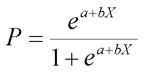
So, to limit the predicted value within (0 – 1) range, you apply a sigmoid transformation on the RHS of the linear regression equation. $$Y = a + b_1X_1 + b2X_2 + .. + b_nX_n + ϵ$$ becomes, $$P(Y=1) = sigmoid(a + b_1X_1 + b_2X_2 + .. + b_nX_n)$$ where sigmoid function of x is: $$sigmoid(x) = \frac{e^x}{1 + e^x}$$
By applying the sigmoid function, the mathematical equation can be generalized as:  where, a is the intercept and b is the slope matrix for all the X’s. Once the equation is formed, it can be used to predict the probability of (Y=1) when only the X is known. Collectively, they are called regression coefficients.
2. Data Exploration
For this implementation, I would be using the Churn Modelling Data. The goal is to predict if the person has churned out or not based on their various features and demographics. You can find the dataset here Let’s see how to do it in Julia.
Import Packages and setup environment
Importing all the packages in the first cell is always a good practice. So let’s load the packages here itself and enable printing max of 1000 columns in the Jupyter cell.
# Import Packages
using Pkg
using DataFrames
using CSV
using Plots
using GLM
using StatsBase
using Lathe
using MLBase
using ClassImbalance
using ROCAnalysis

# Enable printing of 1000 columns
ENV["COLUMNS"] = 1000
Load Data
Read the data using CSV.file function and later convert it to DataFrame object
# Read the file using CSV.File and convert it to DataFrame
df = DataFrame(CSV.File("../Data/Churn_Modelling.csv"))
first(df,5)
 The dependent variable that we want to predict is in the last column (‘exited’). The first column is row numbers, the rest of it are potential X variable (predictors).
Before directly jumping to the model building, exploring the data is important. You should check what’s the size of the data frame if it contains some missing values or outliers.’
Summary of the dataframe
# Summary of dataframe
println(size(df))
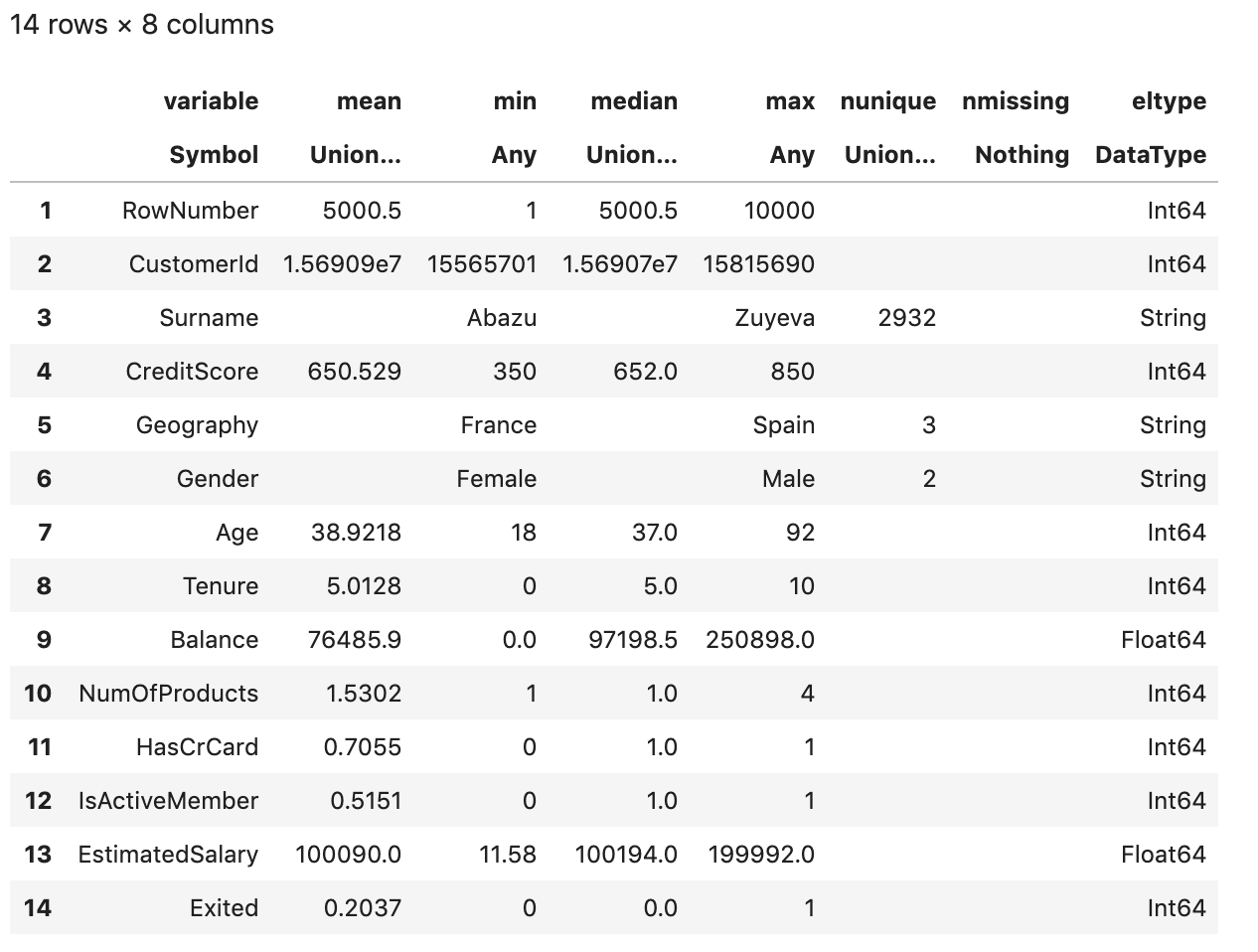
describe(df)
#> (10000, 14)
 There aren’t any missing values in the data set. Let’s check the column names of the data frame. It’s a good practice to avoid spaces, special characters in the column names.
# Check column names
names(df)
Output:
#> 14-element Array{Symbol,1}:
#>  :RowNumber
#>  :CustomerId
#>  :Surname
#>  :CreditScore
#>  :Geography
#>  :Gender
#>  :Age
#>  :Tenure
#>  :Balance
#>  :NumOfProducts
#>  :HasCrCard
#>  :IsActiveMember
#>  :EstimatedSalary
#>  :Exited
Column names are not having spaces and special characters. It’s good to go data set. Now let’s count the number of target classes or Y variable in the data set.
Check Class Imbalance
# Count the classes
countmap(df.Exited)
Output:
#> Dict{Int64,Int64} with 2 entries:
#>  0 => 7963
#>  1 => 2037
The data is quite imbalanced. You need to handle the class imbalance before modeling. But wait you must be thinking why should you do that. Right ? Let’s try that out. I won’t handle it now itself and go ahead with modeling. You yourself will get to know the problem it causes.
3. Data Preprocessing
Data Preprocessing is one of the most important steps in model building. Let’s look at the categorical columns.
One Hot Encoding
One hot encoding is a process of converting categorical variables into a form (numerical columns) that could be fed into ML algorithms to do a better job in prediction. 3 categorical columns are present in the dataset.
These columns need to be handled.
The surname column is having 2932 unique values, so it’s not a good idea to encode it. Rather let’s drop it and encode Gender and Geography columns.
# One hot encoding
Lathe.preprocess.OneHotEncode(df,:Geography)
Lathe.preprocess.OneHotEncode(df,:Gender)
select!(df, Not([:RowNumber, :CustomerId,:Surname,:Geography,:Gender,:Male]))
first(df,5)

Train/Test Split
Split the data to train and test set.
# Train test split
using Lathe.preprocess: TrainTestSplit
train, test = TrainTestSplit(df,.75);
4. Model Building
Let’s build the logistic regression model using the “GLM” package. It’s very similar to the “GLM” package in R. In order to build a logistic regression, family needs to choosen as `Binomial().
# Train logistic regression model
fm = @formula(Exited ~ CreditScore + Age + Tenure + Balance + NumOfProducts + HasCrCard + IsActiveMember + EstimatedSalary + Female + France + Spain)
logit = glm(fm, train, Binomial(), ProbitLink())
StatsModels.TableRegressionModel{GeneralizedLinearModel{GLM.GlmResp{Array{Float64,1},Binomial{Float64},ProbitLink},GLM.DensePredChol{Float64,LinearAlgebra.Cholesky{Float64,Array{Float64,2}}}},Array{Float64,2}}

Exited ~ 1 + CreditScore + Age + Tenure + Balance + NumOfProducts + HasCrCard + IsActiveMember + EstimatedSalary + Female + France + Spain

Coefficients:
───────────────────────────────────────────────────────────────────────────────────────
                        Coef.  Std. Error       z  Pr(>|z|)     Lower 95%     Upper 95%
───────────────────────────────────────────────────────────────────────────────────────
(Intercept)      -1.80953      0.166821    -10.85    <1e-26  -2.1365       -1.48257
CreditScore      -0.000527878  0.00018281   -2.89    0.0039  -0.000886178  -0.000169577
Age               0.0427277    0.00170782   25.02    <1e-99   0.0393804     0.0460749
Tenure           -0.012596     0.00611342   -2.06    0.0394  -0.0245781    -0.000613941
Balance           1.41012e-6   3.36287e-7    4.19    <1e-4    7.51014e-7    2.06923e-6
NumOfProducts    -0.0416691    0.0312514    -1.33    0.1824  -0.102921      0.0195825
HasCrCard        -0.0134524    0.0388497    -0.35    0.7291  -0.0895965     0.0626916
IsActiveMember   -0.572557     0.0368047   -15.56    <1e-53  -0.644692     -0.500421
EstimatedSalary   1.67597e-7   3.0991e-7     0.54    0.5886  -4.39815e-7    7.7501e-7
Female            0.306624     0.0356497     8.60    <1e-17   0.236751      0.376496
France           -0.402329     0.0447782    -8.98    <1e-18  -0.490092     -0.314565
Spain            -0.444951     0.0527071    -8.44    <1e-16  -0.548255     -0.341647
───────────────────────────────────────────────────────────────────────────────────────
Let’s check the performance of the model on the test data which it has never seen.
5. Model Predictions and Evaluation
# Predict the target variable on test data
prediction = predict(logit,test)
Output:
#> 2517-element Array{Union{Missing, Float64},1}:
#>  0.14156472154989325
#>  0.3554447785320442
#>  0.2336139031086097
#>  0.10289516595621737
#>  ⋮
#>  0.05003927571881817
#>  0.3315500629769058
The prediction of glm model is the probability score of class 1. It needs to classified as 0 or 1. Generally, the threshold for classifying the probability is chosen as 0.5.
Let’s convert it to classes i.e. 0 or 1. The probability score less than 0.5 would be treated as 0 and the probability score greater than 0.5 would be treated as 1.
# Convert probability score to class
prediction_class = [if x < 0.5 0 else 1 end for x in prediction];

prediction_df = DataFrame(y_actual = test.Exited, y_predicted = prediction_class, prob_predicted = prediction);
prediction_df.correctly_classified = prediction_df.y_actual .== prediction_df.y_predicted
Output:
#> 2517-element BitArray{1}:
#>  0
#>  0
#>  0
#>  1
#>  1
#>  ⋮
#>  1
#>  0
Accuracy
The Accuracy of a model is the total number of classes predicted correctly by the model.
# Accuracy Score
accuracy = mean(prediction_df.correctly_classified)
#> 0.8029400079459674
An accuracy score of 81% is a good score. But wait, by just looking at the accuracy can you say the model is good? Not convinced? Let’s check another matrix i.e. confusion matrix
Confusion Matrix
Confusion matrix is a table that is often used to evaluate the performance of a classification model.
To know more about the performance metrices of a classification model, refer to Top 15 Evaluation Metrics for Classification Models You can use confusion matrix function to compute the confusion matrix.
But it doesn’t work with class 0. Either change the class 0 to 2 or use a different function. Let’s use the roc function from the MLBase library. It provides positive, negative, true positive, true negative, false positive, and false negative values.
# confusion_matrix = confusmat(2,prediction_df.y_actual, prediction_df.y_predicted)
confusion_matrix = MLBase.roc(prediction_df.y_actual, prediction_df.y_predicted)
Output:
#> ROCNums{Int64}
#>   p = 525
#>   n = 1992
#>   tp = 104
#>   tn = 1917
#>   fp = 75
#>   fn = 421
By looking at the confusion matrix you must have got to know about the problem in the current model. If not, no worries, I will explain it. The model is predicting class 0, most of the time.
It has failed to predict the class 1. The count of false positive is around 4+ times than the true positive. Which proves that the model has failed miserably to predict the class 1.
Let’s look at another very important metric to check the performance of model
ROC
Receiver Operating Characteristics curve is the evaluation metric used to evaluate the classification model based on its predictive power to predict class one’s accuracy and class zero’s accuracy.
In fact, the area under the ROC curve can be used as an evaluation metric to compare the efficacy of the models. Use ‘pyimport’ function from Pycall package to import any python package to julia.
# Import sklearn.metrics to julia
using PyCall
sklearn = pyimport("sklearn.metrics")
Let’s plot the ROC curve using ‘roc_curve’ from ‘sklearn.metrics’ from python. It returns 3 outputs – false positive rate, true positive rate, and thresholds
# Compute false positive rate, true positive rate and thresholds
fpr, tpr, thresholds = sklearn.roc_curve(prediction_df.y_actual, prediction_df.prob_predicted)
Output:
#> ([0.0, 0.000502008032128514, 0.000502008032128514, 0.001004016064257028, 0.001004016064257028, 0.0025100401606425703, 0.0025100401606425703, … #> 0.022445711657822828, 0.016646074957291052, 0.01661423013991524, 0.005148611901203348])
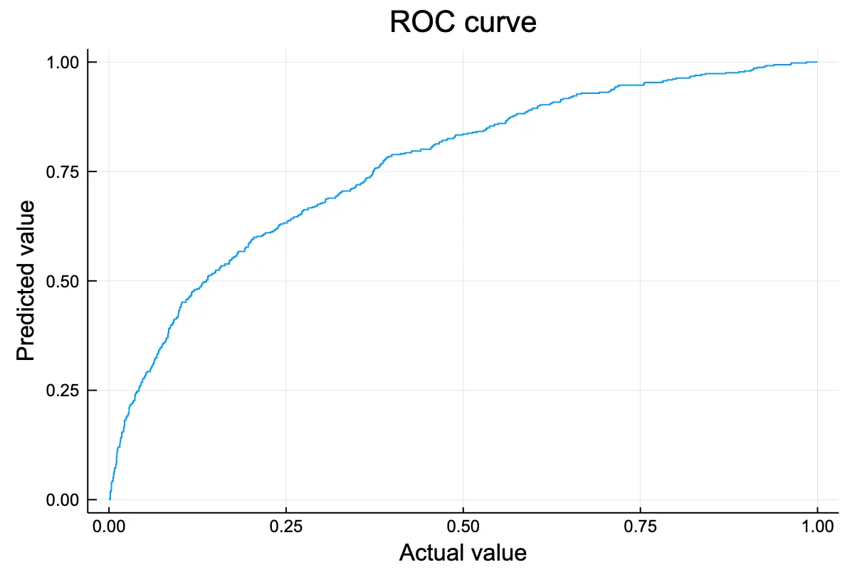
ROC curve is nothing but the curve or plot between false positive rate and true positive rate. False positive rate being the y-axis and true positive rate being the x-axis. Use plot function
# Plot ROC curve
plot(fpr, tpr)
title!("ROC curve")
 Ideally the curve should be close to the y-axis line and top line of the x-axis, but it’s far from it. That means it is not a good model. This is because of the high class imbalance. i.e. while training the data, most of the data points were having class 0. Let’s see how to fix this issue and handle class imbalance
6. Handling Class Imbalance
By now, you know the problems caused by class imbalance. Now I will use a technique smote to handle class imbalance. Refer to Complete introduction to logistic regression to read about more about class imbalance and techniques to handle it. Firstly count the number of classes present in the original data.
# Count the classes
countmap(df.Exited)
Output:
#> Dict{Int64,Int64} with 2 entries:
#>   0 => 7963
#>   1 => 2037
Now let’s use smote function to handle the class imbalance.
X2, y2 =smote(df[!,[:CreditScore,:Age ,:Tenure, :Balance, :NumOfProducts, :HasCrCard, :IsActiveMember, :EstimatedSalary, :Female , :France, :Spain]], df.Exited, k = 5, pct_under = 150, pct_over = 200)
df_balanced = X2
df_balanced.Exited = y2;

df = df_balanced;

# Count the classes
countmap(df.Exited)
#> Dict{Int64,Int64} with 2 entries:
#>   0 => 6111
#>   1 => 6111
It has undersampled the datapoints with class 0 upsampled the datapoints with class 1. Now let’s repeat the steps of model building and check the confusion matrix
# Train test split
train, test = TrainTestSplit(df,.75);

# Model Building
fm = @formula(Exited ~ CreditScore + Age + Tenure + Balance + NumOfProducts + HasCrCard + IsActiveMember + EstimatedSalary + Female + France + Spain)
logit = glm(fm, train, Binomial(), ProbitLink())

# Predict the target variable on test data
prediction = predict(logit,test)

# Convert probability score to class
prediction_class = [if x < 0.5 0 else 1 end for x in prediction];

prediction_df = DataFrame(y_actual = test.Exited, y_predicted = prediction_class, prob_predicted = prediction);
prediction_df.correctly_classified = prediction_df.y_actual .== prediction_df.y_predicted


# Accuracy Score
accuracy = mean(prediction_df.correctly_classified)
print("Accuracy of the model is : ",accuracy)

# Confusion Matrix
confusion_matrix = MLBase.roc(prediction_df.y_actual, prediction_df.y_predicted)
Output:
#> Accuracy of the model is : 0.7098908369169699

#> ROCNums{Int64}
#>   p = 1530
#>   n = 1493
#>   tp = 1073
#>   tn = 1073
#>   fp = 420
#>   fn = 457
The accuracy of the model has reduced to 71.4%. But overall the confusion matrix has improved. The cases of true positive and true positive are almost equal.
The cases for false positive and false negative are also almost equal. Hence you can call it a better model as compared to the previous one.
Conclusion
I have covered the basic concepts about logistic regression and it’s implementation in Julia. Please note that it’s very important to handle the class imbalance before going for the model building in logistic regression. Next I will see you with more Data Science oriented topics in Julia. Read more about Julia here


