

Explore the fundamentals of sampling and sampling distributions in statistics. Dive deep into various sampling methods, from simple random to stratified, and uncover the significance of sampling distributions in detail.

In this blog post we will learn
- What is Sampling?
- Why Sample?
- Types of Sampling Methods
3.1. Simple Random Sampling (SRS)
3.2. Stratified Sampling
3.3. Cluster Sampling
3.4. Systematic Sampling
3.5. Convenience Sampling
3.6. Quota Sampling - Simple demonstration of different sampling methods using Python
- What is a Sampling Distribution?
5.1. Simulate and visualize the sampling distribution of the sample mean using Python
5.2. Key Concepts in Sampling Distributions
5.3. Importance of Sampling Distributions - Conclusion
1. What is Sampling?
Sampling refers to the process of selecting a subset (or a sample) from a larger set (often called a population). Instead of collecting data from every individual in the population (which can be time-consuming and costly), researchers typically collect data from a sample and then use that sample to make inferences about the larger population.
For example, if we wanted to know the average height of all adult men in a country, instead of measuring every single man, we could measure a sample of them and then estimate the average height for the entire group.
2. Why Sample?
Sampling has a host of benefits:
- Cost-effective: It’s often cheaper to collect data from a sample than from an entire population.
- Time-saving: Sampling can save a considerable amount of time.
- Feasibility: In some cases, it’s virtually impossible to survey an entire population.
- Accuracy: If done correctly, sampling can provide accurate estimates of population parameters.
3. Types of Sampling Methods
3.1. Simple Random Sampling (SRS)
Definition: Every individual in the population has an equal chance of being selected.
Example: Imagine a bowl containing 100 unique lottery tickets. If you were to close your eyes and pick out 10 tickets one at a time, you’re engaging in simple random sampling.
3.2. Stratified Sampling
Definition: The population is divided into non-overlapping groups (or strata) based on a particular characteristic, and then a random sample is taken from each group.
Example: Let’s say you’re researching study habits among high school students across freshmen, sophomores, juniors, and seniors. Instead of picking randomly from the whole school, you first divide students by grade level and then randomly pick an equal number from each grade. This ensures representation from all grades.
3.3. Cluster Sampling
Definition: The population is divided into clusters (often geographically), and then a random sample of clusters is chosen. All or a random sample of members from those selected clusters will be surveyed.
Example: Imagine you want to survey households in a large city. The city is divided into different neighborhoods (clusters). Instead of sampling households from the entire city, you randomly select a few neighborhoods and then survey all households (or a random sample of them) within those selected neighborhoods.
3.4. Systematic Sampling
Definition: Every $k$ th individual is selected from a list or sequence.
Example: You have a list of 1,000 customers and want to select 50 for a survey. To do this, you might select every 20th customer from the list (1,000 divided by 50 equals 20). So you’d survey the 20th, 40th, 60th customer, and so on.
3.5. Convenience Sampling
Definition: The sample is chosen based on what is easy or convenient, rather than any systematic or random method.

Example: A street interviewer stops passers-by at a mall entrance to ask about their shopping preferences. Here, the sample consists of whoever happens to be at that particular entrance at that time – it’s convenient, but not necessarily representative of all shoppers.
3.6. Quota Sampling
Definition: The researcher ensures equal or proportionate representation of subjects depending on certain characteristics, but the selection within those categories might be non-random.
Example: If you’re surveying voters’ intentions before an election and you know the gender distribution is 50% male and 50% female, you might ensure that out of 100 surveyed individuals, 50 are male and 50 are female. However, how you select those 50 males and females might not be random.
4. Simple demonstration of different sampling methods using Python
import pandas as pd
import numpy as np

# Create a sample DataFrame for demonstration
data = {
    'ID': range(1, 101),  # IDs for 100 individuals
    'Age': np.random.randint(15, 65, 100),  # Random ages between 15 and 65
    'Grade': np.random.choice(['Freshman', 'Sophomore', 'Junior', 'Senior'], 100)  # Random school grades
}
df = pd.DataFrame(data)

df.head()
| ID | Age | Grade | |
|---|---|---|---|
| 0 | 1 | 48 | Junior |
| 1 | 2 | 23 | Sophomore |
| 2 | 3 | 62 | Sophomore |
| 3 | 4 | 24 | Freshman |
| 4 | 5 | 44 | Junior |
# 1. Simple Random Sampling (SRS)
srs_sample = df.sample(n=10)  # Get 10 random rows from the DataFrame

print("Simple Random Sampling (SRS) Sample:")
srs_sample
Simple Random Sampling (SRS) Sample:
| ID | Age | Grade | |
|---|---|---|---|
| 89 | 90 | 38 | Freshman |
| 98 | 99 | 21 | Junior |
| 76 | 77 | 37 | Junior |
| 97 | 98 | 37 | Junior |
| 28 | 29 | 18 | Junior |
| 6 | 7 | 16 | Junior |
| 32 | 33 | 44 | Freshman |
| 24 | 25 | 56 | Junior |
| 94 | 95 | 33 | Senior |
| 8 | 9 | 24 | Senior |
# 2. Stratified Sampling
strat_sample = df.groupby('Grade').apply(lambda x: x.sample(n=2)).reset_index(drop=True)  # Get 2 samples from each grade

print("\nStratified Sampling Sample:")
strat_sample
Stratified Sampling Sample:
| ID | Age | Grade | |
|---|---|---|---|
| 0 | 10 | 59 | Freshman |
| 1 | 97 | 52 | Freshman |
| 2 | 12 | 17 | Junior |
| 3 | 98 | 37 | Junior |
| 4 | 88 | 51 | Senior |
| 5 | 30 | 34 | Senior |
| 6 | 72 | 33 | Sophomore |
| 7 | 35 | 30 | Sophomore |
# 3. Cluster Sampling
clusters = df.groupby(df.index // 10)  # Create 10 clusters
selected_clusters = clusters.apply(lambda x: x if np.random.rand() < 0.2 else None).dropna()  # Select 20% of clusters

print("\nCluster Sampling Sample:")
selected_clusters
Cluster Sampling Sample:
| ID | Age | Grade | ||
|---|---|---|---|---|
| 5 | 50 | 51 | 22 | Senior |
| 51 | 52 | 50 | Sophomore | |
| 52 | 53 | 33 | Sophomore | |
| 53 | 54 | 25 | Freshman | |
| 54 | 55 | 30 | Senior | |
| 55 | 56 | 46 | Senior | |
| 56 | 57 | 28 | Freshman | |
| 57 | 58 | 48 | Senior | |
| 58 | 59 | 26 | Junior | |
| 59 | 60 | 25 | Junior |
# 4. Systematic Sampling
k = len(df) // 10
sys_sample = df.iloc[::k].head(10)

print("\nSystematic Sampling Sample:")
sys_sample
Systematic Sampling Sample:
| ID | Age | Grade | |
|---|---|---|---|
| 0 | 1 | 48 | Junior |
| 10 | 11 | 46 | Junior |
| 20 | 21 | 41 | Freshman |
| 30 | 31 | 34 | Junior |
| 40 | 41 | 24 | Sophomore |
| 50 | 51 | 22 | Senior |
| 60 | 61 | 52 | Freshman |
| 70 | 71 | 28 | Senior |
| 80 | 81 | 60 | Freshman |
| 90 | 91 | 18 | Freshman |
# 5. Convenience Sampling
# Here, we'll just take the first 10 rows. In real-world scenarios, this would be akin to surveying whoever comes first.
conv_sample = df.head(10)

print("\nConvenience Sampling Sample:")
conv_sample
Convenience Sampling Sample:
| ID | Age | Grade | |
|---|---|---|---|
| 0 | 1 | 48 | Junior |
| 1 | 2 | 23 | Sophomore |
| 2 | 3 | 62 | Sophomore |
| 3 | 4 | 24 | Freshman |
| 4 | 5 | 44 | Junior |
| 5 | 6 | 52 | Sophomore |
| 6 | 7 | 16 | Junior |
| 7 | 8 | 50 | Sophomore |
| 8 | 9 | 24 | Senior |
| 9 | 10 | 59 | Freshman |
# 6. Quota Sampling
# Let's say we have a quota to sample 3 individuals from each grade.
quota_sample = df.groupby('Grade').apply(lambda x: x.sample(n=3)).reset_index(drop=True)

print("\nQuota Sampling Sample:")
quota_sample
Quota Sampling Sample:
| ID | Age | Grade | |
|---|---|---|---|
| 0 | 47 | 36 | Freshman |
| 1 | 33 | 44 | Freshman |
| 2 | 10 | 59 | Freshman |
| 3 | 96 | 39 | Junior |
| 4 | 5 | 44 | Junior |
| 5 | 59 | 26 | Junior |
| 6 | 30 | 34 | Senior |
| 7 | 88 | 51 | Senior |
| 8 | 78 | 56 | Senior |
| 9 | 53 | 33 | Sophomore |
| 10 | 8 | 50 | Sophomore |
| 11 | 64 | 16 | Sophomore |
5. What is a Sampling Distribution?
A sampling distribution is the distribution of a statistic (like the mean or proportion) based on all possible samples of a given size from a population. It tells us how much we would expect our sample statistic to vary from one sample to another.
For instance, if we were to repeatedly draw different samples of 100 men from our earlier example and calculate the average height for each sample, the distribution of those sample means would be the sampling distribution of the mean.
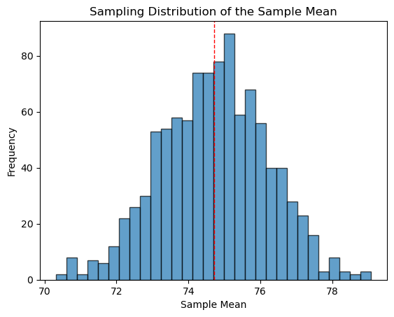
5.1. Simulate and visualize the sampling distribution of the sample mean using Python
In this example:
- We’ve created a population with a mean of 75 and a standard deviation of 15.
- We then repeatedly (1,000 times) drew random samples (each of size 100) from this population.
- For each sample, we computed its mean and stored it.
- Finally, we visualized the distribution of these sample means.
import numpy as np
import pandas as pd
import matplotlib.pyplot as plt

# Generating the population data
np.random.seed(0)
population_data = np.random.randn(10000) * 15 + 75  # Let's say the population data is normally distributed with mean 75 and standard deviation 15.

# Simulate the sampling distribution of the sample mean
num_samples = 1000
sample_size = 100
sample_means = []

for _ in range(num_samples):
    sample = np.random.choice(population_data, size=sample_size, replace=False)
    sample_means.append(np.mean(sample))

# Plotting
plt.hist(sample_means, bins=30, edgecolor='k', alpha=0.7)
plt.title("Sampling Distribution of the Sample Mean")
plt.xlabel("Sample Mean")
plt.ylabel("Frequency")
plt.axvline(x=np.mean(sample_means), color='r', linestyle='dashed', linewidth=1)
plt.show()
5.2. Key Concepts in Sampling Distributions
Central Limit Theorem (CLT): For a sufficiently large sample size, the sampling distribution of the sample mean will be approximately normal, regardless of the population’s distribution. This is a powerful property that allows us to make statistical inferences.
To learn more about Central Limit Theorem refer to this blog post Central Limit Theorem
Standard Error (SE): It measures the dispersion or variability of sample statistics from one sample to the next. A smaller SE indicates that our sample statistic (like the mean) is more consistent across different samples.
5.3. Importance of Sampling Distributions
Sampling distributions are crucial for hypothesis testing and confidence interval estimation. Knowing how our sample statistic behaves (its distribution) under repeated sampling allows us to:
- Assess the likelihood of observing our sample results if some null hypothesis were true.
- Gauge the precision of our sample estimates.
6. Conclusion
Sampling and its associated distribution provide the foundation for much of inferential statistics. By understanding these concepts, we are better equipped to make informed decisions based on sample data. As always, the key lies in choosing the right sampling method and ensuring that our sample is representative of the larger population.

