Introduction

Singular Value Decomposition, commonly known as SVD, is a powerful mathematical tool in the world of data science and machine learning. SVD is primarily used for dimensionality reduction, information extraction, and noise reduction. In this post, we will delve deep into the world of SVD, understand its mechanics, and witness its applications with the help of examples.

Importance in Data Science

1. Dimensionality Reduction: The larger the data, the harder it is to process and visualize. Using SVD, we can reduce the dimensions of our data while preserving most of its variance. This is the principle behind techniques like Principal Component Analysis (PCA).

2. Noise Reduction: In many scenarios, datasets have noise. SVD helps in decomposing the matrix in a way that separates signal from noise.

3. Recommendation Systems: The famous Netflix Prize competition saw the application of SVD in recommendation systems. The algorithm decomposes the user-item interaction matrix to predict missing values representing user ratings.

What is Singular Value Decomposition?

SVD is a method for decomposing a matrix. For a given matrix $A$, it can be decomposed into three matrices $U$, $Σ$, and $V^T$, such that:

$ A = UΣV^T $

Given a matrix $ A $ of dimensions $ m \times n $, the SVD decomposes it into three matrices:

1. $ U $: An $ m \times m $ orthogonal matrix, called the “left singular” matrix.
2. $ Σ $: An $ m \times n $ diagonal matrix, with non-negative real numbers on the diagonal. The values on the diagonal are the “singular values” and are usually ordered in decreasing order.
3. $ V^T $: An $ n \times n $ orthogonal matrix, where $ V^T $ is the transpose of $ V $, called the “right singular” matrix.

So, the decomposition can be represented as:
$ A = U Σ V^T $

The columns of $ U $ are called the left singular vectors, the columns of $ V $ are called the right singular vectors, and the non-zero values in $ Σ $ are the singular values of $ A $.

Simple Example:

Let’s compute the SVD for a small matrix:
$ A = \begin{bmatrix} 4 & 0 \\ 0 & 3 \end{bmatrix} $

Using a software tool or library (like MATLAB, NumPy in Python, etc.), you can compute the SVD of this matrix. Doing so, you’d find:

$ U = \begin{bmatrix} 1 & 0 \\ 0 & 1 \end{bmatrix} $

$ Σ = \begin{bmatrix} 4 & 0 \\ 0 & 3 \end{bmatrix} $

$ V^T = \begin{bmatrix} 1 & 0 \\ 0 & 1 \end{bmatrix} $

Notice in this simple example that $ A $ is already a diagonal matrix, so the SVD just gives us back the matrix $ A $ itself in $ Σ $, and $ U $ and $ V^T $ are the identity matrices.

For non-diagonal matrices, the SVD decomposition will look more complex. But the main idea is the same: you can decompose any matrix into three other matrices, representing orthogonal transformations and scaling.

The diagonal elements of $Σ$ are known as singular values and are non-negative. The columns of $U$ and $V^T$ are orthonormal eigenvectors of $AA^T$ and $A^TA$, respectively.

# Singular Value Decomposition
import numpy as np

# Define the matrix A
A = np.array([[4, 0], 
              [0, 3]])

# Compute the SVD
U, Sigma, Vt = np.linalg.svd(A)

print("Matrix A:")
print(A)
print("\nU matrix:")
print(U)
print("\nSigma matrix (as a diagonal matrix):")
print(np.diag(Sigma))
print("\nVt matrix:")
print(Vt)

Matrix A:
[[4 0]
 [0 3]]

U matrix:
[[1. 0.]
 [0. 1.]]

Sigma matrix (as a diagonal matrix):
[[4. 0.]
 [0. 3.]]

Vt matrix:
[[1. 0.]
 [0. 1.]]

Example: SVD in Action

Using SVD for Image Compression

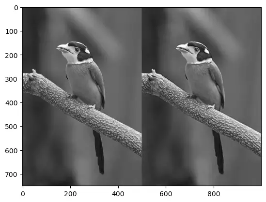
One of the fascinating applications of SVD is image compression. Let’s take an example of compressing a grayscale image.

1. Import Necessary Libraries:

import numpy as np
import matplotlib.pyplot as plt
from skimage import io, color

1. Load and Display the Image:

image_url = "https://upload.wikimedia.org/wikipedia/commons/b/b2/JPEG_compression_Example.jpg"

#image_url = "https://encrypted-tbn0.gstatic.com/images?q=tbn:ANd9GcQcYkADf34lxq-cL9rJqWQ0PT0SwFk5r_FZVQ&usqp=CAU"
image = io.imread(image_url, as_gray=True)
plt.imshow(image, cmap='gray')
plt.show()

1. Perform SVD on the Image:

U, S, Vt = np.linalg.svd(image, full_matrices=False)

1. Compress the Image:
   To compress the image, retain only the first $k$ singular values, and corresponding vectors.

k = 50
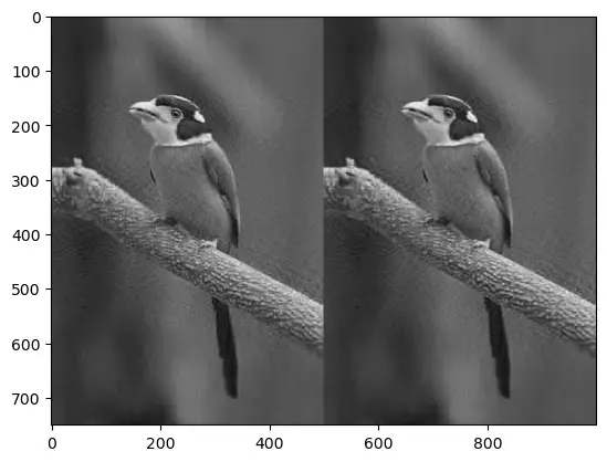
compressed_image = np.dot(U[:, :k], np.dot(np.diag(S[:k]), Vt[:k, :]))

1. Display Compressed Image:

plt.imshow(compressed_image, cmap='gray')
plt.show()

By using only 50 singular values, the image is compressed while preserving the overall structure and features.

Conclusion

Singular Value Decomposition is undoubtedly a gift to the data science community. From enabling machine learning models to work efficiently on massive datasets to helping in image and signal processing, the applications are vast and impactful.

By understanding and harnessing the power of SVD, data scientists can extract meaningful insights from data and craft effective algorithms.