T Test (Students T Test) is a statistical significance test that is used to compare the means of two groups and determine if the difference in means is statistically significant.
In this one, you’ll understand when to use the T-Test, the different types of T-Test, math behind it, how to determine which test to choose in what situation and why, how to read from the t-tables, example situations and how to apply it in R and Python.
 T Test (Students T Test) – Understanding the math and how it works. Photo by Parker Coffman.
Contents
Introduction
T Test is one of the foundational statistical tests. It is used to compare the means of two groups and determine if the difference is statistically significant. It is a very common test often used in data and statistical analysis.
So when to use the T-Test?
Let’s suppose, you have measurements from two different groups, say, you are measuring the marks scored by students from a class you attended special coaching versus those who did not. And you want to determine if the scores of those who attending the coaching is significantly higher than those who did not. You can use the T-Test to determine this.
However, depending on how the groups are chosen and how the measurements were made you will have to choose a different type of T-Test for different situations. You will see more such examples coming up.
By the end of this you will know:
- How the Student’s T Test got its name
- What is the T-Test
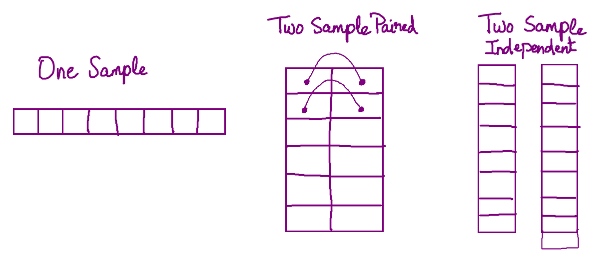
- Three Types of T-Tests
- How to pick the right T-Test to use in various situations
- Example Situations of when to use which test
- Formula of T-Statistic (in various situations)
- T Test Solved Exercise
Story Behind the T-Test
T-Test was first invented by ‘William Sealy Gosset’, when he was working at Guinness Brewery. The original goal was to select the best barley grains from small samples, when the population standard deviation was not known.
If Mr. Gossett invented it, why is it called Student’s T-Test instead of ‘Gosett’s T-Test’?
It’s said that Guinness didn’t want him to reveal some sort of industry secret which may be detrimental from a business point of view. However, they allowed him to publish it under a different name.
So he published his work in a paper title ‘Biometrika’ in 1908 under the pseudoname ‘Student’ and the name caught on. As a result this test is often referred to as ‘Student’s T Test’.
So, effectively this test has been around for more than a century and is in active use today.
This test assumes that the test statistic, which is often the ‘sample mean’, should follow a normal distribution. Let’s look at the types of T-Tests.
What are the three types of T-Tests?
-
- One Sample T-Test
Tests the null hypothesis that the population mean is equal to a specified value `μ` based on a sample mean `x̄`.Input:
Small numeric array (vector) and hypothesized population mean.Output:
T-Statistic, P value.When to use (example):
Test if the mean weight of adult male mice is 10g (population mean), given a numeric array of mouse weights.
- One Sample T-Test
-
- Two Sample Independent T-Test
Tests the null hypothesis that two sample means x̄1 and x̄2 are equal. Compares the means of two numeric variables obtained from two independent groups.Input:
Two numeric arrays which may or may not be of the same size. They belong to two different groups.Output:
T-Statistic, P value.When to use (example):
Test of the mean weight of mangoes from Farm A equals mean weight of mangoes from Farm B.
- Two Sample Independent T-Test
- Two Sample Dependent T-Test (aka Paired T-Test)
Compare the means of two numeric variables of same size where the observations from the two variables are paired. Typically, it may be from the same entity before and after a treatment, where treatment could be showing a commercial and the measured value could be opinion score about a brand.Input:
Two numeric arrays of same size and observations from the two samples are paired.Output:
T-Statistic, P-ValueWhen to use (example):
Given the numeric ratings of same menu items from two different restaurants (rated by same connoisseur), determine which restaurant’s food tastes better?
How to perform a T Test?
The main part of performing the T-Test is in computing the T Statistic, which is the test statistic in this case.
The way you compute the t-statistic is different depending on the type of t-test. Let’s see how to compute it one by one.
1. One-Sample Student’s t-test:
You perform a one sample T Test when you want to test if the population mean is of a specified value μ given by a sample mean x̄.
Let me put it plainly: you have a sample of observations for which you know the mean (sample mean), and you want to test if the sample came from a population with given (hypothesized) mean.
Step 1: Define the Null and Alternate Hypothesis
H0 (Null Hypothesis): Sample Mean (x̄) = Hypothesized Population Mean(μ)
H1 (Alternate Hypothesis): Sample Mean (x̄) != Hypothesized Population Mean(μ)
Step 2: Compute the T statistic
Use the following formula to compute the t-statistic:
$$t = \frac{x̄ – μ}{s/\sqrt{n}}$$
where, x̄=sample mean, μ=population mean, n=sample size, s=sample standard error.
The only difference with the z-statistic formula is that instead of population standard deviation, it uses the sample’s standard error.
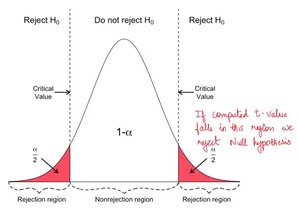
Step 3: Lookup T critical and check if computed T statistic falls in rejection region.
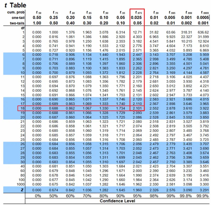
Based on the degrees of freedom (n-1) and the alpha level (typically 0.05), lookup the critical T value from the T-Table. If the absolute value of the computed T-statistic is greater than the critical T-value, that is, it falls in the rejection region, then we reject the null hypothesis that the population mean is of the specified value.
Alternately, you can check the output P-value. P-value is typically an output from the software as a result of the T Test. If the P-value is lesser that the significance level (typically 0.05), then reject the null hypothesis and conclude that the population mean is different from what is stated.
The t-critical score is dependent on:
1. Degrees of freedom, which in this case is sample size minus 1 (n-1).
2. Chosen significance level (default: 0.05).
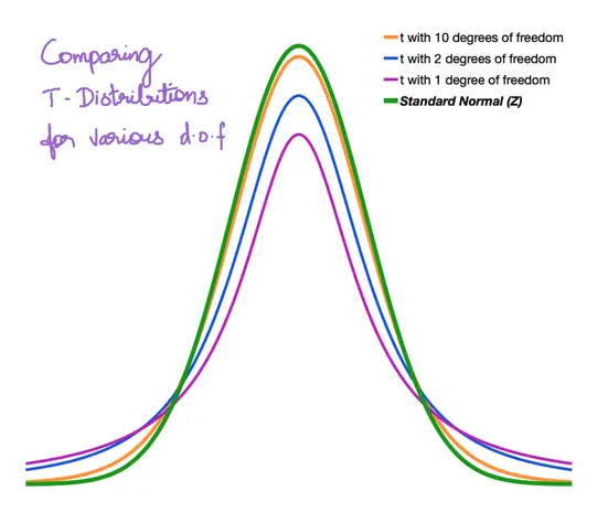
The shape of the T Distribution depends on the number of degrees of freedom (d.o.f), which is in turn dependent on the number of observations in the sample. It is simply (n-1). T distribution usually has fatter tail, which gets narrower as the degree of freedom increases.
As the number of observations (or d.o.f) increase, the T distribution becomes closer in shape to the standard normal distribution.
2. Independent Two-Sample T-Test:
When trying to compare two samples with a two-sample t-test, you can think of the t-test as a ratio of signal (sample means) to noise (sample variability).
$$t = \frac{signal}{noise} = \frac{difference \; in \; means}{sample \; variability} = \frac{\bar{x_1} – \bar{x_2}}{\sqrt{\frac{s_1^2}{n_1} + \frac{s_2^2}{n_2}}}$$
where, x̄1, x̄2 = sample means, s_1^1, s_2^2 = sample variances and n_1, n_2 = sample sizes.
Once t-statistic is computed, we then compare it to the critical t-score for a given degrees of freedom df and significance level (α).
How to compute the degrees of freedom?
Since the sample sizes of the two samples can be unequal with different variances, determining the degrees of freedom is not as straight forward as you saw in 1-sample t-test.
The formula for calculating df was given by Welch-Satterthwaite as shown below.
$$df = \frac{\left(\frac{s_1^2}{n_1} + \frac{s_2^2}{n_2}\right)^2}{\frac{1}{n_1-1}\left( \frac{s_1^2}{n1}\right)^2 + {\frac{1}{n_2-1}\left( \frac{s_2^2}{n2}\right)^2}}$$
If you have approximately same variances in each sample, though that may not always be the case, the above equation can be generalized as below:
$$df = n1 + n2 – 2$$
Once degree of freedom is calculated, for the given alpha level (say 0.05) you will lookup the T-table for the critical T value. Then, based on the T-critical, see of the computed T value falls in the rejection region. If it does, we reject the null hypothesis and understand that the means from the two samples are not the same.
Let’s solve an example problem.
T-Test Example Exercise
Problem Statement
A global fast food chain wants to venture into a new city by setting up a store in a popular mall in the city. It has shortlisted 2 popular locations A and B for the same and wants to choose one of them based on the number of foot falls per week.
The company has obtained the data for the same and wants to know which of the two locations to choose and if there is significant difference between the two.
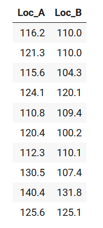
Here’s how the footfalls per day (in 1000’s) looks like for 10 randomly chosen days:
Solution
First, let’s compare the sample means.
$$\bar{x}_{Loc A} = 121.72$$
$$\bar{x}_{Loc B} = 112.84$$
x̄_LocA – x̄_LocB = 8.88
Looks like, Location A gets 8.88k more footfalls on an average over a period of 10 days.
However, the average number of footfalls is in these locations in much more and tend to vary on a day to day basis. So, the question remains: Is an additional avg footfall of 8.88k measured over 10 days, enough to say that Loc A receives different footfalls than Loc B? Is it statistically significant?
How to find this out?
Let’s begin by framing the null and alternate hypothesis.
Step 0: Identify the type of T Test.
Well, here are the facts: There are two samples. Each sample contains the number of footfalls but since both are random samples the observations are not paired. That is, the number of footfalls of 116.2 in location A does not correspond to 110.0 in location B because they may not be captured on the same day. So, the observations are not paired, as a result, the T-Test to perform is the Two Sample Independent T Test.
Step 1: Frame the null and alternate hypothesis
Null Hypothesis H0: x̄_LocA = x̄_LocB
Alternate Hypothesis H1: x̄_LocA != x̄_LocB
Step 2: Degrees of freedom
Since this is a 2 sample t-Test, the degrees of freedom = 10 + 10 – 2 = 18
Ideally we should use Welch-Satterthwaite’s formula. But for simplicity of manual calculation, I am using this one for now.
Step 3: Compute the t-Statistic
Let’s start by computing the variance
Variance of Loc_A = 80.508
Variance of Loc_B = 95.584
$$t = \frac{\bar{x_1} – \bar{x_2}}{\sqrt{\frac{s_1^2}{n_1} + \frac{s_2^2}{n_2}}} = \frac{8.88}{\sqrt{\frac{80.51}{10} + \frac{95.58}{10}}} = 2.1161$$
Step 4: Lookup the critical value from t-table
If the computed T-statistic falls in the rejection
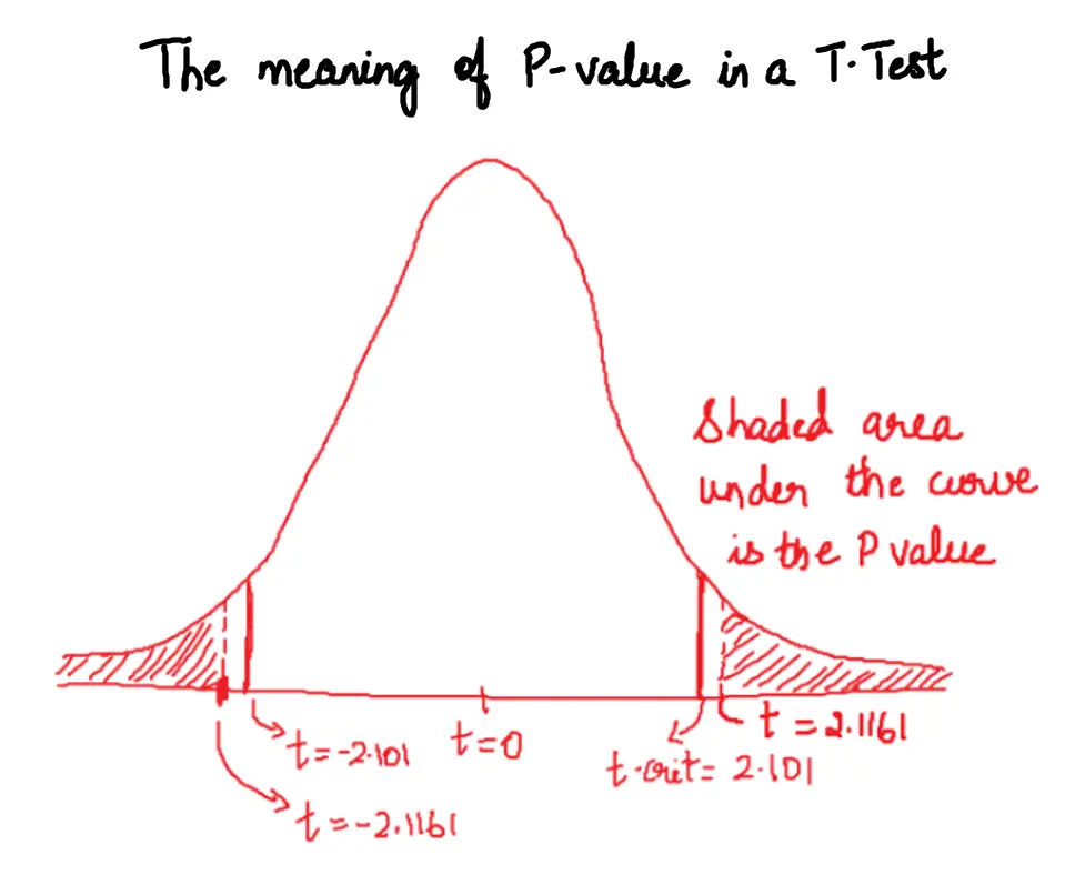
Since its a two-tailed test with 18 degrees of freedom. And assuming a default 95% confidence, the critical value from the t-table is 2.101
In our case, the t-statistic (2.1161) > t-critical (2.101)
This means, the t-statistic does falls in the rejection zone and so, we reject the null hypothesis and conclude that the means are in fact different.
How to implement t-test in R and Python?
Below is a reproducible code to implement the t-test for the problem we just discussed.
How to do T Test In R?
df <- read.csv("https://raw.githubusercontent.com/selva86/datasets/master/footfalls.csv")

t.test(df[, 'Loc_A'], df[, 'Loc_B'], paired=FALSE)

#>     Welch Two Sample t-test
#> data:  df$Loc_A and df$Loc_B
#> t = 2.1161, df = 17.869, p-value = 0.04864
#> alternative hypothesis: true difference in means is not equal to 0
#> 95 percent confidence interval:
#>   0.05916631 17.70083369
#> sample estimates:
#> mean of x mean of y
#>    121.72    112.84
# Compute P Value (area to the right and left extremities of the computed T-Statistic)
2 * pt(-2.1161, 18)
#> 0.048532
How to do T Test In Python?
from scipy.stats import ttest_ind
import pandas as pd
df = pd.read_csv("https://raw.githubusercontent.com/selva86/datasets/master/footfalls.csv")
tscore, pvalue = ttest_ind(df.Loc_A, df.Loc_B)
print("t Statistic: ", tscore)
print("P Value: ", pvalue)

#> t Statistic:  2.1161
#> P Value:  0.0485
# Compute P Value explicitly (Python)
from scipy.stats import t
t_dist = t(18)
2 * t_dist.cdf(-2.1161)
#> 0.048532
Conclusion
We have seen a lot of details both T-Test and the different types. Next, we will go through each type of T-Test in more detail with worked out examples. Stay tuned.


