Spline Interpolation – How to find the polynomial curve to interpolate missing values

Written by Selva Prabhakaran | 3 min read

Spline interpolation is a special type of interpolation where a piecewise lower order polynomial called spline is fitted to the datapoints. That is, instead of fitting one higher order polynomial (as in polynomial interpolation), multiple lower order polynomials are fitted on smaller segments.

This can be implemented in Python.

You can do non-linear spline interpolation in Python using the pandas library by setting method='spline' in the interpolate() method of the series object.

By adjusting the order parameter, you can control the curviness of the splines.

How to do Spline interpolation in Python?

First, let’s implement it with pandas using the interpolate method of a pandas series object. To use spline interpolation, you need to set the method to ‘spline’ and set the ‘order’ as well.

Let’s see an example based on the train fare example we saw in linear interpolation example.

python

import pandas as pd

fare = {'first_class':100, 
        'second_class':np.nan, 
        'third_class':60, 
        'open_class':20}

ser = pd.Series(fare)
ser

python

first_class     100.0
second_class      NaN
third_class      60.0
open_class       20.0
dtype: float64

We make sure the ‘x’ (index in this case) is in ascending order. So, we use ‘reset_index()’ method.

python

ser.reset_index().interpolate(method='spline', order=2)

	index	0
0	first_class	100.000000
1	second_class	86.666667
2	third_class	60.000000
3	open_class	20.000000

What if you have the data as a Dataframe?

Works as well. But take care of the index.

python

# apply interpolate on a pandas dataframe.
data = pd.DataFrame(ser,columns=['Fare'])
data.reset_index().interpolate(method='spline', order=2)

	index	Fare
0	first_class	100.000000
1	second_class	86.666667
2	third_class	60.000000
3	open_class	20.000000

Cubic spline interpolation using scipy

python

from scipy.interpolate import CubicSpline
import numpy as np

X = [0, 1, 2, 3, 4, 5]
Y = [8.1, 10.2, 15.4, 24.6, 29.8, 31.9]
x = 2.5

# make sure X is in ascending order
def make_ascending(X,Y):    
    if np.any(np.diff(X) < 0):
        sorted_index = np.argsort(X).astype(int)
        X = np.array(X)[sorted_index]
        Y = np.array(Y)[sorted_index]
    return X, Y

X, Y = make_ascending(X,Y)        

# learn the CubicSpline function
f = CubicSpline(X, Y, bc_type='natural')

# Predict Y given x 
f(x)

python

array(20.)

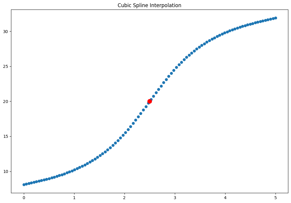
Let’s plot how the entire function will look like.

python

from scipy.interpolate import CubicSpline
import numpy as np
import matplotlib.pyplot as plt

X = [0, 1, 2, 3, 4, 5]
Y = [8.1, 10.2, 15.4, 24.6, 29.8, 31.9]

# Make ascending
X, Y = make_ascending(X,Y)   

# Learn the cubic spline function
f = CubicSpline(X, Y, bc_type='natural')

# predict for the entire range of X
x = np.linspace(np.min(X), np.max(X), 100)
y = f(x)

Plot it

python

# Plot
plt.scatter(x, y)
plt.scatter(x=2.5, y=f(2.5), c='red', s=100)
plt.title('Cubic Spline Interpolation')
plt.show()

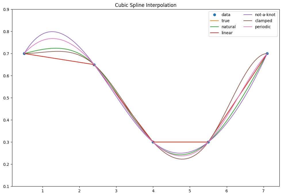
Comparing linear interpolation and various cubic spline interpolation

There are multiple methods within CubicSpline function from scipy. Let’s plot how they fit the data

python

# imports
import matplotlib.pyplot as plt
import numpy as np
from scipy.interpolate import CubicSpline, interp1d
plt.rcParams['figure.figsize'] =(12,8)

x = [.5, 2.4, 4.0, 5.5, 7.1]
y = [.7, .65, .3, .3, .7]

# apply cubic spline and linear interpolation
cs = CubicSpline(x, y, bc_type='natural')
cs_nak = CubicSpline(x, y, bc_type='not-a-knot')
cs_per = CubicSpline(x, y, bc_type='periodic')
cs_clm = CubicSpline(x, y, bc_type='clamped')
linear_int = interp1d(x,y)

# generate all possible X
X = np.linspace(np.min(x), np.max(x), 100)

# plot data
plt.plot(x, y, 'o', label='data')
plt.plot(x, y, label='true')

# Natural spline
plt.plot(X, cs(X), label="natural")

# Linear
plt.plot(X, linear_int(X),  label="linear")

# Not a Knot
plt.plot(X, cs_nak(X), label="not-a-knot")

# Clamped
plt.plot(X, cs_clm(X), label="clamped")

# Periodic
plt.plot(X, cs_per(X), label="periodic")

# plot elements
plt.ylim(.1, .9)
plt.legend(loc='upper right', ncol=2)
plt.title('Cubic Spline Interpolation')
plt.show()